theory - Unsupervised Domain Adaptation

• Domain Adaptation
  • Unsupervised Domain Adaptation
• Transfer Learning & Deep Domain Adaptation
  • Discrepancy-based methods
    • Discrepancy
    • Domain distribution Alignment Layers (?)
  • Adversarial-based methods
  • Reconstruction-based methods

Domain Adaptation

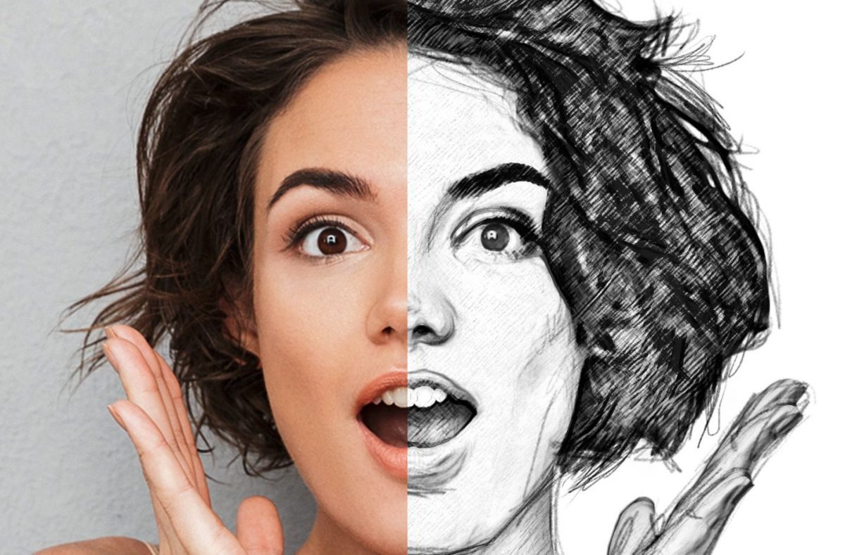
in traditional machine learning the main assumptions is that train and test data come from the same domain; but in real world many time the training differs from the test data, this phenomena is called domain shift (time & environmental changes, different modalities, synthetic to real images, cad to real images and others).

the most naive approach is to finetune the network on the different data, of course this is possible if and only if we have annotated data on the new test data, so in this case it requires annotations at any new setting.

Unsupervised Domain Adaptation

In this scenario we have labelled data source but we are not interested in the performance in the source domain but only interested in the performance in the target domain where instead the data are not annotated.

$D_{S} = {(x_{i}^{S}, y_{i}^{S})}_{i=1}^{N}$

$D_{T} = {(x_{j}^{T})}_{j=1}^{M}$

we can have situations in which we have different features spaces but the same target space (eg. same classes) but also situations in which we also have different label spaces. .

Transfer Learning & Deep Domain Adaptation

Transfer learning is a research problem in machine learning that focuses on storing knowledge gained while solving one problem and applying it to a different but related problem (!= fine tuning).

the domain is the set of data that are coherent in the same aspect (same distribution), we typically have the source and the target domain ($D_{S}, D_{T}$).

Three main categories:

1. Discrepancy-based methods: align domain data representations with statistical measures.
2. Adversarial-based methods: generally involve a domain discriminator to enforce domain confusion (very much like how GAN works).
3. Reconstruction-based methods: uses an auxiliary reconstruction task to ensure a “good” domain-invariant feature representation.

Discrepancy-based methods

These methods are also called deep domain confusion, the main idea is that we force the network to produce two similar feature representation of the two different domain.

Discrepancy

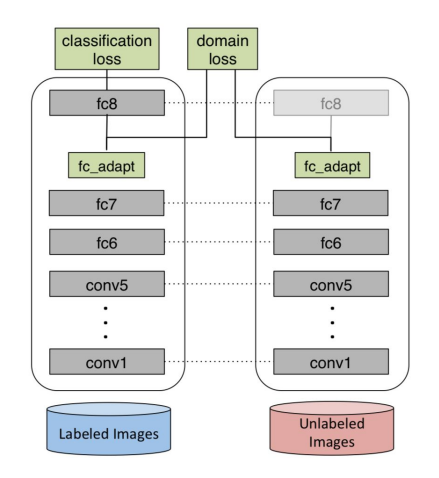
We propose a new CNN architecture which introduces an adaptation layer and an additional domain confusion loss, to learn a representation that is both semantically meaningful and domain invariant. We additionally show that a domain confusion metric can be used for model selection to determine the dimension of an adaptation layer and the best position for the layer in the CNN architecture.

Optimizing for domain invariance, therefore, can be considered equivalent to the task of learning to predict the class labels while simultaneously finding a representation that makes the domains appear as similar as possible. This principle forms the essence of our proposed approach. We learn deep representations by optimizing over a loss which includes both classification error on the labeled data as well as a domain confusion loss which seeks to make the domains indistinguishable.

We propose a new CNN architecture, outlined in Figure 1, which uses an adaptation layer along with a domain confusion loss based on maximum mean discrepancy (MMD) to automatically learn a representation jointly trained to optimize for classification and domain invariance.

We show that our domain confusion metric can be used both to select the dimension of the adaptation layers, choose an effective placement for a new adaptation layer within a pretrained CNN architecture, and fine-tune the representation.

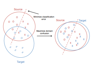
Directly training a classifier using only the source data often leads to overfitting to the source distribution, causing reduced performance at test time when recognizing in the target domain. Our intuition is that if we can learn a representation that minimizes the distance between the source and target distributions, then we can train a classifier on the source labeled data and directly apply it to the target domain with minimal loss in accuracy. To minimize this distance, we consider the standard distribution distance metric, MMD (Maximum Mean Discrepancy) where we have two network that crate the feature representation for both domains and then we add a loss function that force this network to produce similar features map using the following loss:

$L = L_{c}(X_{S}, y_{S}) + \lambda MMD^{2}(X_{S}, X_{T})$

where the first loss represent the classification loss while the second represent the domain distance loss that could be calculated using the MMD which is a way to understand how two very high dimensional matrix are similar (distance between the source data and the target data).

There are two model selection choices that must be made to add our adaptation layer and the domain distance loss. We must choose where in the network to place the adaptation layer and we must choose the dimension of the layer. We use the MMD metric to make both of these decisions. Evaluating adaptation layer placement, Choosing the adaptation layer dimension.

Fine-tuning with domain confusion regularization wowever, we need to set the regularization hyperparameter $\lambda$. Setting $\lambda$ too low will cause the MMD regularizer have no effect on the learned representation, but setting $\lambda$ too high will regularize too heavily and learn a degenerate representation in which all points are too close together. We set the regularization hyperparameter to $\lambda = 0.25$, which makes the objective primarily weighted towards classification, but with enough regularization to avoid overfitting.

Domain distribution Alignment Layers (?)

Learn domain-agnostic representations by acting inside the architecture of the given deep network, they are derived from batch norm:

$DA_{BN}(x,k)= \gamma \cdot \frac{x - \mu_{k} } {\sqrt{\sigma^{2} + \epsilon}} + \beta$

Adversarial-based methods

As the training progresses, the approach promotes the emergence of “deep” features that are (i) discriminative for the main learning task on the source domain and (ii) invariant with respect to the shift between the domains. We show that this adaptation behaviour can be achieved in almost any feed-forward model by augmenting it with few standard layers and a simple new gradient reversal layer. The resulting augmented architecture can be trained using standard backpropagation.

Our goal is to embed domain adaptation into the process of learning representation, so that the final classification decisions are made based on features that are both discriminative and invariant to the change of domains, i.e. have the same or very similar distributions in the source and the target domains. In this way, the obtained feed-forward network can be applicable to the target domain without being hindered by the shift between the two domains

We thus focus on learning features that combine (i) discriminativeness and (ii) domain-invariance. This is achieved by jointly optimizing the underlying features as well as two discriminative classifiers operating on these features: (i) the label predictor that predicts class labels and is used both during training and at test time and (ii) the domain classifier that discriminates between the source and the target domains during training. While the parameters of the classifiers are optimized in order to minimize their error on the training set, the parameters of the underlying deep feature mapping are optimized in order to minimize the loss of the label classifier and to maximize the loss of the domain classifier. The latter encourages domain-invariant features to emerge in the course of the optimization.

Our approach is generic as it can be used to add domain adaptation to any existing feed-forward architecture that is trainable by backpropagation. In practice, the only non-standard component of the proposed architecture is a rather trivial gradient reversal layer that leaves the input unchanged during forward propagation and reverses the gradient by multiplying it by a negative scalar during the backpropagation.

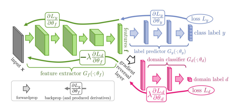
We now define a deep feed-forward architecture that for each input x predicts its label $y \in Y$ and its domain label $d \in {0,1}$. We decompose such mapping into three parts. We assume that the input x is first mapped by a mapping $G_{f}$ (a feature extractor) to a D-dimensional feature vector $f \in R^{d}$. The feature mapping may also include several feed-forward layers and we denote the vector of parameters of all layers in this mapping as $\theta_{f}$ , i.e. $f = G_{f}(x, \theta_{f})$. Then, the feature vector f is mapped by a mapping $G_{y}$ (label predictor) to the label y, and we denote the parameters of this mapping with $\theta_{y}$ . Finally, the same feature vector f is mapped to the domain label $d$ by a mapping $G_{d}$ (domain classifier) with the parameters $\theta_{d}$

During the learning stage, we aim to minimize the label prediction loss on the annotated part (i.e. the source part) of the training set, and the parameters of both the feature extractor and the label predictor are thus optimized in order to minimize the empirical loss for the source domain samples. This ensures the discriminativeness of the features $f$ and the overall good prediction performance of the combination of the feature extractor and the label predictor on the source domain. At the same time, we want to make the features $f$ domain-invariant.

Measuring the dissimilarity of the distributions $S_{f}$ and $T_{f}$ is however non-trivial, given that f is high-dimensional, and that the distributions themselves are constantly changing as learning progresses. One way to estimate the dissimilarity is to look at the loss of the domain classifier $G_{d}$, provided that the parameters $\theta_{d}$ of the domain classifier have been trained to discriminate between the two feature distributions in an optimal way.

This observation leads to our idea. At training time, in order to obtain domain-invariant features, we seek the parameters $\theta_{f}$ of the feature mapping that maximize the loss of the domain classifier (by making the two feature distributions as similar as possible), while simultaneously seeking the parameters $\theta_{d}$ of the domain classifier that minimize the loss of the domain classifier. In addition, we seek to minimize the loss of the label predictor.

The parameter $\lambda$ controls the trade-off between the two objectives that shape the features during learning.

y introducing a special gradient reversal layer (GRL) defined as follows. The gradient reversal layer has no parameters associated with it (apart from the meta-parameter $\lambda$, which is not updated by backpropagation). During the forward propagation, GRL acts as an identity transform. During the backpropagation though, GRL takes the gradient from the subsequent level, multiplies it by - $\lambda$ and passes it to the preceding layer. Implementing such layer using existing object-oriented packages for deep learning is simple, as defining procedures for forwardprop (identity transform), backprop (multiplying by a constant), and parameter update (nothing) is trivial.

We can then define the objective “pseudo-function” of ($\theta_{f}$ , $\theta_{y}$, $\theta_{d}$) that is being optimized by the stochastic gradient descent within our method:

$ E(\theta_{f}, \theta_{y}, \theta_{d}) = \sum_{i=1..N} L_{y}(G_{y}(G_{f}(x_{i}; \theta_{f}); \theta_{y}), y_{i}) + \sum_{i=1..N} L_{d}(G_{d}(R_{\lambda}(G_{f}(x_{i}; \theta_{d})); \theta_{y}), y_{i}) $

Reconstruction-based methods

novel unsupervised domain adaptation algorithm based on deep learning for visual object recognition. Specifically, we design a new model called Deep ReconstructionClassification Network (DRCN), which jointly learns a shared encoding representation for two tasks: i) supervised classification of labeled source data, and ii) unsupervised reconstruction of unlabeled target data. In this way, the learnt representation not only preserves discriminability, but also encodes useful information from the target domain. Our new DRCN model can be optimized by using backpropagation similarly as the standard neural networks.

Domain adaptation attempts to deal with dataset bias using unlabeled data from the target domain so that the task of manual labeling the target data can be reduced. Unlabeled target data provides auxiliary training information that should help algorithms generalize better on the target domain than using source data only.

We consider a solution based on learning representations or features from raw data. Ideally, the learned feature should model the label distribution as well as reduce the discrepancy between the source and target domains. We hypothesize that a possible way to approximate such a feature is by (supervised) learning the source label distribution and (unsupervised) learning of the target data distribution. This is in the same spirit as multi-task learning in that learning auxiliary tasks can help the main task be learned better. The goal of this paper is to develop an accurate, scalable multi-task feature learning algorithm in the context of domain adaptation.

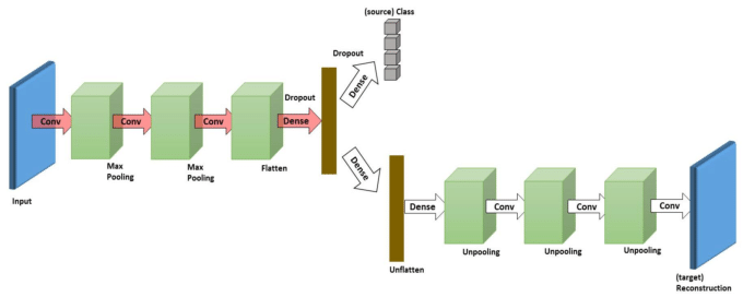
We propose Deep Reconstruction-Classification Network (DRCN), a convolutional network that jointly learns two tasks: i) supervised source label prediction and ii) unsupervised target data reconstruction. The encoding parameters of the DRCN are shared across both tasks, while the decoding parameters are separated. The aim is that the learned label prediction function can perform well on classifying images in the target domain – the data reconstruction can thus be viewed as an auxiliary task to support the adaptation of the label prediction. Learning in DRCN alternates between unsupervised and supervised training, which is different from the standard pretraining-finetuning strategy.

However, our proposed method undertakes a fundamentally different learning algorithm: finding a good label classifier while simultaneously learning the structure of the target images.

Typically, $L_{c}$ is of the form cross-entropy loss and $L_{r}$ is of the form squared loss. Our aim is to solve the following objective:

$min \ \lambda L_{c}^{n_{s}} ({\Theta_{enc}, \Theta_{label}}) +(1-\lambda) L_{c}^{n_{t}} ({\Theta_{enc}, \Theta_{dec}})$

where $0 < \lambda < 1$ is a hyper-parameter controlling the trade-off between classification and reconstruction. The objective is a convex combination of supervised and unsupervised loss functions.

The stopping criterion for the algorithm is determined by monitoring the average reconstruction loss of the unsupervised model during training – the process is stopped when the average reconstruction loss stabilizes

The architecture and learning setup: The DRCN architecture used in the experiments is adopted from. The label prediction pipeline has three convolutional layers: 100 5x5 filters (conv1), 150 5x5 filters (conv2), and 200 3x3 filters (conv3) respectively, two max-pooling layers of size 2x2 after the first and the second convolutional layers (pool1 and pool2), and three fully-connected layers (fc4, fc5,and fc out) – fc out is the output layer. The number of neurons in fc4 or fc5 was treated as a tunable hyper-parameter in the range of [300, 350, …, 1000], chosen according to the best performance on the validation set. The shared encoder genc has thus a configuration of conv1-pool1-conv2- pool2-conv3-fc4-fc5. Furthermore, the configuration of the decoder gdec is the inverse of that of genc. Note that the unpooling operation in gdec performs by upsampling-by-duplication: inserting the pooled values in the appropriate locations in the feature maps, with the remaining elements being the same as the pooled values. We employ ReLU activations in all hidden layers and linear activations in the output layer of the reconstruction pipeline. Updates in both classification and reconstruction tasks were computed via RMSprop with learning rate of $10^{-4}$ and moving average decay of 0.9. The control penalty $\lambda$ was selected according to accuracy on the source validation data – typically, the optimal value was in the range [0.4, 0.7].