theory - Recurrent Nets

• Recurrent Neural networks
  • Character prediction example
  • Vanilla RNN
  • Backpropagation trough time (BPTT)
  • Gated port and LSTM
  • Gated Recurrent Unit (GRU)
    • Bi-directional RNNs

Recurrent Neural networks

So far, we focused mainly prediction problems with fixed-size inputs and outputs. We discussed the flexibility of CNN to address a wide range of tasks. But what if the input and/or output is a variable-length sequence? many tasks require this as document classification, sentiment analysis (text analysis) and image captioning (Given an image, produce a sentence describing its contents().

We have three scenario in which we can use RNN:

1. Multiple2Single as in text classification we have an input which consists of many tokens and we output a single output.

2. Single2Multiple as in image captioning where we have one image and the output is a sequence, as a text describing the image.

3. Multiple2Multiple as in text translation where we have multiple input and multiple output.

in all this situations the contextual information is captured by some hidden state, denoted with $h$.

The idea of unfolding a recursive or recurrent computation into a computational graph that has a repetitive structure, typically corresponding to a chain of events. Unfolding this graph results in the sharing of parameters across a deep network structure.

Both the recurrent graph and the unrolled graph have their uses. The recurrent graph is succinct. The unfolded graph provides an explicit description of which computations to perform. The unfolded graph also helps to illustrate the idea of information flow forward in time (computing outputs and losses) and backward in time (computing gradients) by explicitly showing the path along which this information flows.

To design a sequence modeling we need to:

1. handle variable-length sequences
2. Track long-term dependencies
3. Maintain information about order
4. Share parameters across the sequence

Character prediction example

We will have recurrent model that allow to predict the next character, i want to predict the word given context from the previous character. Since the characters are limited numbers we can thing to use one-hot encoding for translate the digits into vectors. In any case there the need to provide some form of representation of the text to the model.

Then first set of weights connected the input to the hidden representations (input to the hidden representation) and ten we have the weights hidden state ( previous hidden representation to current hidden representation) and lastly we have the hidden layer that maps to the output target (hidden layer to the output layer (easy ffd network)).

Vanilla RNN

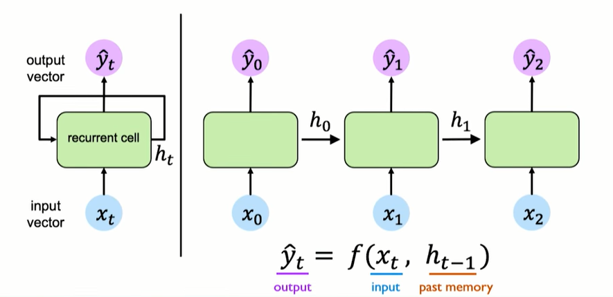
RNN has some cycle inside allowing to represent a hidden state hat well be used for the prediction, it depended on the hidden representation of the previous state and the input itself. we take the input $x$ and the previous hidden state $h_{t-1}$ and i want the hidden representation at time time t, to do this use simply use an affine transformation plus a non linear function (typically tangent despite the fact that we have some derivative that are very small if we are far away from the origin).

$h_{t} = f_{W}(x_{t}, h_{t-1}) $ $h_{t} = tanh(W_{hh}^{T} h_{t-1}, W_{xh}^{T} h_{x_{t}}) $

where $h_{t}$ os the new state, $x_{t}$ is the input at time $t$ and $h_{t-1}$ is the old state. Rnn have a this state $h_{t}$, that is updated at each ime step as sequence is processed;

To train this i compose multiple RNN cell and the output of the hidden state is the input for the new cell together with the new input; we typically use soft-max so to have probabilities. The parameters between this RNN cell are shared among the network.

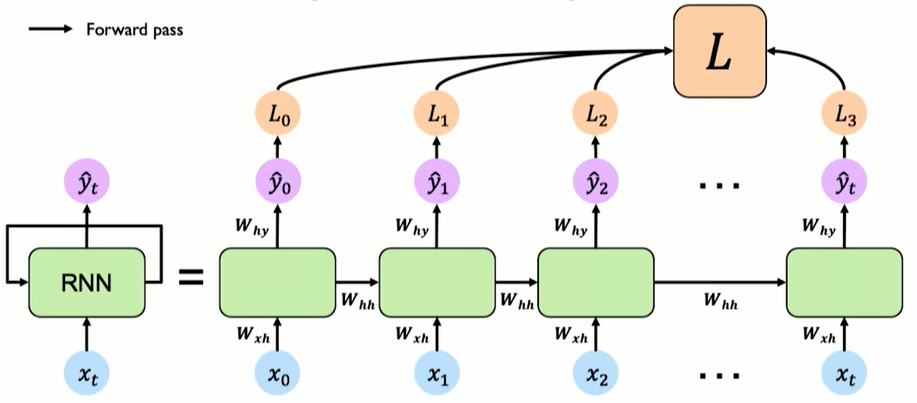
the same function and set of parameters ad used at every time step. Importantly this function is parametrize by the weights W, this set of weights is the same across all the time steps that are be considered in the sequence (as well as the function).

The weight matrices that are applied to the hidden state is different from the one of the matrix that process the input matrices but it is important that these same weight matrices are re used all trough the network, the $w_{xh}$ and $w_{hh}$ are the same al over the network that is why in RN there are shared parameters.

The problem is that somehow to compute the derivative we have to sum and take into account all the contributions of all the different time step. We also need a loss function for training a RNN, for doing that we create a loss for each of the individual output at that time step and creating a common Loss summing them up.

{width=550}

Backpropagation trough time (BPTT)

Our forward pass is little different, we compute individual loss and summing them together, to backpropagate now we have to backpropagate error individually across all the time steps from where we are to the beginning. Errors flow back in time to the beginning of the sequence.

The problem is that somehow to compute the derivative we have to sum and take into account all the contributions of all the different time step. If we follow all the derivation we discover that the chain rule get more complicated because we end up in a summation (because we have to take in count all the previous time step). The fact that we have this summation and that the one of this term is the product of multiple terms means that i’m multiplying the derivative of the activation time number that are close to zero.

Between each time step we need to perform this matrix multiplication, so we have to taking the loss of the internal state requires many many matrix multiplication and this is problematic:

1. Gradient exploding: we may many high vale the gradients could explode (simple solution is to gradient clipping so to scale back bigger gradient)

2. Gradient vanishing: but also opposite problem where we have vanishing gradients so to slow learning (pushing the model to focus on short dependencies (still high gradient) but not too far dependencies).

for computing the gradients we use the backpropagation trough time (BPTT), The unfolded network (used during forward pass) is treated as one big feed-forward network that accepts the whole time series as input: The weight updates are computed for each copy in the unfolded network, then summed (or averaged) and applied to the RNN weights (backward pass).

the problems in vanilla BPTT is that if input sequences are comprised of thousands of timesteps, then this will be the number of derivatives required for a single update weight update. This can cause weights to vanish or explode and make slow learning and model skill poor, moreover BPTT can be computationally expensive as the number of timesteps increases.

How we make this computation feasible? we can try to use a truncated BPTT. the solution is an heuristic process, we will take a sequence of k1 timesteps and consider the associate input output pairs; we will use the k1 and k2 timesteps for updating the network.

This approach influence how fast the training is, how well we capture temporal dependencies and gradient issues (trade off between the three).

Gated port and LSTM

the most effective sequence models used in practical applications are called gated RNNs. These include the long short-term memory and networks based on the gated recurrent unit. Like leaky units, gated RNNs are based on the idea of creating paths through time that have derivatives that neither vanish nor explode. Leaky units did this with connection weights that were either manually chosen constants or were parameters. Gated RNNs generalize this to connection weights that may change at each time step. Leaky units allow the network to accumulate information (such as evidence for a particular feature or category) over a long duration. However, once that information has been used, it might be useful for the neural network to forget the old state. For example, if a sequence is made of sub-sequences and we want a leaky unit to accumulate evidence inside each sub-subsequence, we need a mechanism to forget the old state by setting it to zero. Instead of manually deciding when to clear the state, we want the neural network to learn to decide when to do it. This is what gated RNNs do.

a very popular is the LSTM and the main intuition is to modify the vanilla RNN cell by adding a new cell (memory cell) that is still update and having a particular design such that the processing associated to this memory cell will not be subject to non-linearity and avoiding the vanishing gradient (mitigated). The key idea is to add extra variable to update $c_{t}$.

Gradient flow from ct to ct-1 only involves backpropagating through addition and element-wise multiplication, not matrix multiplication or tanh.

The clever idea of introducing self-loops to produce paths where the gradient can flow for long durations is a core contribution of the initial long short-term memory (LSTM) model. A crucial addition has been to make the weight on this self-loop conditioned on the context, rather than fixed. By making the weight of this self-loop gated (controlled by another hidden unit), the time scale of integration can be changed dynamically. In this case, we mean that even for an LSTM with fixed parameters, the time scale of integration can change based on the input sequence, because the time constants are output by the model itself.

one peculiarity of LSTM cell is the presence of a neuron with a self-recurrent connection (connection to itself), and this is what made the model robust; the second peculiar is the set of gates:

1. input gate that will allow to incoming single to alter the state of the memory or cell
2. Output gate can allow the state of the memory cell to have an effect on their neurons
3. Forget gate can modulate the memory cell’s self-recurrent connection, allowing the cell to remove or forget its previous state, as needed.

the key idea is that we have these gates that try to control the information flow;

1. Maintain a cell state (memory cell that is not subject to matrix multiplication or squishing, thereby avoiding gradient decay)
2. use gates to control the flow of information
   • Forget gate gets rid of irrelevant information
   • Store relevant information from current input
   • Selective update cell state
   • Output gate returns a filtered version of the cell state
3. backpropagation trough time with partially uninterrupted gradient flow (it is more stable and mitigate the gradient vanishing reducing the number of mat multiplication).

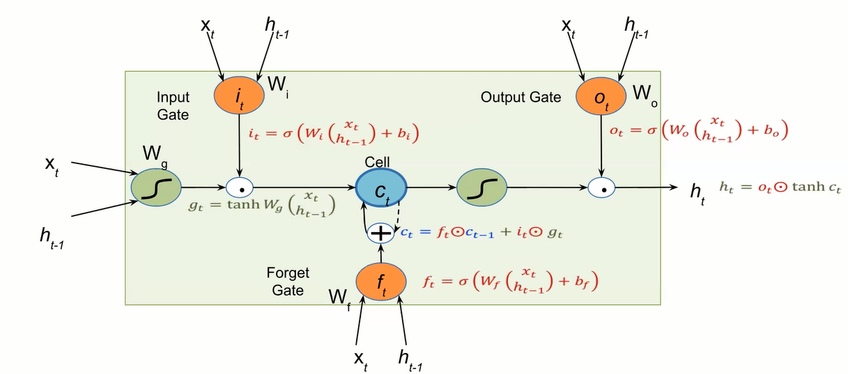
the inner variable ct is recurrently updated with the previous state and with $g_{t}$ which is the output of our non linear-function. I’ll append the first gates the input gates that takes in the input at time step t and the hidden state of the previous cell, the peculiarity is the usage of the sigmoid (because is a gate) that modulate the flow of the information; in fact the $i_{t}$ is multiplied by $g_{t}$ modulating the input. Then we have the output gate that is used to modulate the $c_{t}$ for the next cell and lastly we have the forget gate which is used to indicate how much i want to forget the memory cells into the previous steps.

We will end up having a tangent function a many sigmoid function. And what is making the LSTM robust is that the cell c_{t} only involves backprop trough addition and element-wise multiplication, not matrix multiplication or tahn.

Gated Recurrent Unit (GRU)

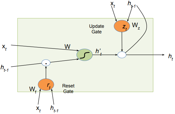
One big improvement for improving LSTM is represented by the GRU that removes one gates, they remove the cell states and proved that by using the reset gate and modifying the update gate we will mitigate the vanishing gradient and using less parameters is in any case better.

GRU get rid of the cell state and use the hidden state to transfer information. it is more compact since it requires only two gates:

1. The reset gate is used from the model to decide how much of the past information to forget.

2. The update gate helps the model to determine how much of the past information (from previous time steps) needs to be passed along to the future.

instead of using ct the similar update is made on ht but still some of the properties for the propagation are needed.

Bi-directional RNNs

Somehow if we are precessing information in a direction we are not really modelling well the dependencies, while we do not create a model for dependencies in other direction.

RNNs can process the input sequence in forward and in the reverse direction.