theory - Generative Models

• Generative Models
  • Implicit density model
    • Generative Adversarial Networks (GAN)
      • Non-Saturating GAN Loss
      • Test loss does not imply quality images
    • Gan zoo
      • DCGAN
    • Evaluation GAN
    • Gan Issues
    • Training Tricks
      • Feature Matching
      • Mini-batch Discrimination
      • Virtual Batch Norm
      • Label & label smoothing
      • Conditional GAN (CGAN)
      • InfoGAN
      • Wasserstein GAN
      • LSGAN
    • Image2Image translation
      • Pix2Pix network
      • CycleGAN
      • Text-To-Image synthesis
    • GAN Summary
  • Non Probabilistic Approach
    • Autoencoders
  • Explicit density model
    • AutoRegressive models
      • PixelRNN
      • PixelCNN
      • AutoRegressive advantages
    • Variation AutoEncoders (VAE)
    • Conditional
    • VAE vs GAN
  • Final comparison

Generative Models

Generative model works in a context of unsupervised learning. in this scenario we do not have labels but we just have data. the main goal is to learn some underlying hidden structure of the data.

One important task in unsupervised learning is density estimation, we want to learn the underlying probability model that generate this data. We want to do that because we want to sample from that model and produce data that are similar in my training set (no need of labels).

the common tasks in unsupervised deep learning are:

1. dimensionality reduction
2. density estimation
3. clustering

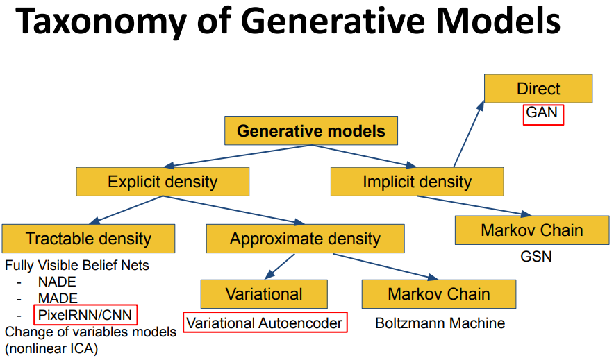
One common taxonomy divided the models into non-probabilistic models (as auto encoders) and probabilist generative models, in this last category we have two possible approaches:

Trying explicitly to learn the distribution of the data or use a smart strategy and use an implicit density estimation .

This model rely only on data, given a huge dataset we want to generate new sample from the same distribution. Given a dataset of faces i want to generate a face. An application could be given training data, generate new samples from same distribution where we know that $training \ data \sim \ p_{data(x)}$ and $p_{data(x)}$ is unknown we want to learn some $p_{model(x)}$ similar to $p_{data(x)}$ where $p_{model(x)}$ is the distribution generated from the model.

For doing that we have two main strategies:

1. Explicit density estimation where we explicitly define and solve for $p_{model(x)}$ figuring out an optimization approach such that the parameters are learned to get close to the $p_{data(x)}$ (which we do not have).

2. Implicit density estimation learn model that can sample from $p_{model(x)}$ without explicitly defining it. I want to learn a model that can sample from the data but i do not need a explicit function for it.

With GAN we can generate images from sample but also art works, translate image domain from another, complex text into image, generate images and so on.

Generative models can be used for simulation and planning (e.g. transform synthetic data into realistic ones) they also can also enable inference of latent representations that can be useful as general features.

Implicit density model

Generative Adversarial Networks (GAN)

Generative Adversarial Networks (GANs) do not consider any explicit density function, they just focus on the ability of the model to sample from a complex high-dimensional training distribution.

Instead of sampling directly from image is to introducing a nn that sample such that you sample from a simple gaussian distribution and this will be passed to the generation network that has the role to translate this simple space in something complex that should resemble the data that we have.

To ensure that the generation is done well we introduce another nn that will try to distinguish between real (from the training dataset) and fake images (generated).

These family of models are called sample generation. The core idea is to sample from a very simple distribution, usually a normal distribution and learn transformation to training distribution with neural network.

We pass a matrix of vector noise to our network generator abd this has the role to generate the random noise into something complex that should resemble the original dataset probability. this is done trough a two-player game where we have two neural nets one is the discriminator which will try to distinguish between real and fake images and a generator that try to fool the discriminator by generating realistic images.

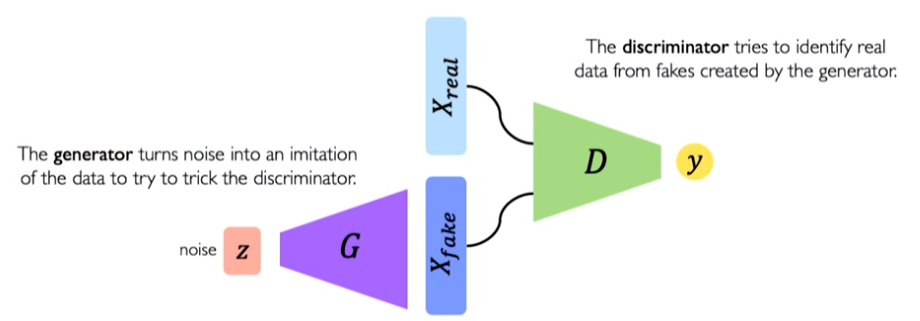
The discriminator will be trained to understand if an image is real or fake while the generator will be pushed to generate image that seems more real to the discriminator.

to train a han we need to train jointly the generator and the discriminator using a min max objective function called adversarial objective.

I have two nn so i want to maximize to respect of the parameter of the discriminator say respect to the real data $E {x} p_{data}$; The second expectation is taken from the sample data $E {x} p_{z}$ because we are passing trough the generator; the discriminator is evaluating the output of the generator:

1. The discriminator maximize such that the probability is close to 1 when i have real data and 0 when is fake data

2. the generator is the opponent and aim to let the discriminator output one when the data are fake.

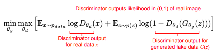
where $z$ is the noise vectors and $G(z)$ is the output of the generator given the noise vector $z$; $D(G(Z))$ is output of the discriminator when given fake generated data or $G(Z)$ and $D(X)$ is the output of the discriminator when given real training data from X.

training gan is very hard, using this naive approach in practice does not work well. When sample is likely fake, we want to improve the generator but the gradient in that case s relatively flat (the model will learn only if it is already good enough to challenge the discriminator).

The generator tries to minimize this function while the discriminator tries to maximize it. Looking at it as a min-max game, this formulation of the loss seemed effective.

The Standard GAN loss function can further be categorized into two parts: Discriminator loss and Generator loss. $log(D(x))$ refers to the probability that the generator is rightly classifying the real image, maximizing $log(1-D(G(z)))$ would help it to correctly label the fake image that comes from the generator.

The discriminator should maximize $Log(D(X))$, and as Log is a monotonic function so $Log(D(X))$ will automatically get maximized if the discriminator maximized $D(X)$. The discriminator needs to maximize $log(1 — D(G(Z)))$, which means it must have to minimize $D(G(Z))$.

in the original paper the procedure that was proposed to train the gan we have gradient ascent on discriminator and gradient descent on generator, they realized that this introduce optimization difficulties.

In practice, it saturates for the generator, meaning that the generator quite frequently stops training if it doesn’t catch up with the discriminator. We will have many update when the generator is already doing something good but at the beginning the gradient is flat so we are not improving much.

Non-Saturating GAN Loss

A subtle variation of the standard loss function is used where the generator maximizes the log of the discriminator probabilities $– log(D(G(z)))$.

instead of performing gradient descent they perform gradient ascent also in the generator.

This change is inspired by framing the problem from a different perspective, where the generator seeks to maximize the probability of images being real, instead of minimizing the probability of an image being fake.

Anyway train two different nn is very difficult.

Test loss does not imply quality images

Another problem is that the learning curve is correlated on what the network is doing, while training GAN with this naive approach did not make the loss related to the quality of the images generated.

Once the training is done we do not need the discriminator anymore, indeed we just keep the generator since we can produce new data from it. Another problem related to that is that the loss is not meaningful for understating if the quality of the generated image is good or not (in term of human understand).

At test time the discriminator is not needed anymore, i just use it for training the generator; at test time i can sample from the simple distribution only the generator.

GAN are very flexible we can create generator and discriminator with different architectures (using lice fully connected layers or conv net). Also the design of the generator/discriminator is very important to create good models.

Gan zoo

DCGAN

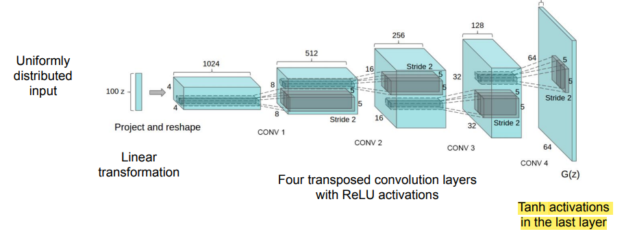
one the first work after the GAN breakthrough, the first questions were related to the architecture to use. the DCGAN proposed some principles for designing convolutional architectures for GANs, first model for large resolution image generation.

The generator was build with a bunch of transposed convolutional layer and used ReLU, batchnorm and Tanh as last layer.

Discriminator architecture

• No pooling, only strided convolutions
• Use Leaky ReLU activations (sparse gradients cause problems for training)
• Use only one FC layer before the soft-max output
• Use batch normalization after most layers

It sample from distribution trough transpose convolution it produces images.

This work as become some much important is because they understand something about the role of the latent space;

If taking the mean of the latent code of different images and perform some arithmetic we produce some images that is able to change only some particular features. By simply doing arithmetic they were able to condition the result of the generated image (e.g man with glasses -man without glasses + woman without glasses = woman with glasses).

The first was the vector arithmetic with faces. For example, a face of a smiling woman minus the face of a neutral woman plus the face of a neutral man resulted in the face of a smiling man. Specifically, the arithmetic was performed on the points in the latent space for the resulting faces. Actually on the average of multiple faces with a given characteristic, to provide a more robust result.

They start playing with latent features, like performing a pose transformation by adding a “turn” vector.

This prove that the latent space is someway organized.

Evaluation GAN

the problem related to GAN are traditionally:

• stability of the GAN
• the choice of the architectures
• lastly when we generate something we have the problem of evaluating the performance.

This is again a problem, whenever we have a generation process then we need a way to evaluate it and since there is an implicit distribution we do not have a proper way to evaluate GAN.

1. Human performance: Human that is asked if the image is real or not for a lot og image.

2. Inception Score: Key idea: generators should produce images with a variety of recognizable object classes. What i would expect from a GAN? i want that the images are various and if i have different objects i’d like that the GAN generate all the objects not a small subsets of it. If i look at the single image i want that the object is well recognize.

following two criteria: 1. A human, looking at each image, would be able to confidently determine what is in there (saliency). 2. A human, looking at a set of various images, would say that the set has lots of different objects (*diversity).

I will do this using distribution, the inception score (because inception was the good classifier at the time). Probability that the object is in the image and the marginal distribution considering the labels.

this classification is done using an image classifier, the main disadvantage is that a GAN that simply memorized the training data, if the GAN learn to copy the training set that already posses diversity and saliency (as it is) i’m not able to detect that the model is overfitting.

The second problem is that if the GAN will outputs a single image per class (mode dropping) could still score well.

1. Fréchet Inception Distance: Let’s compare the statistics of the feature generate by all the network in the real and generated images, if the network as learned similar feature at different levels it means that the GAN is doing a good jobs (comparing statistics in term of first and second order statistics metrics).

   1. Pass generated samples through a classification network and compute activations for a chosen layer.

   2. Estimate multivariate mean and covariance of activations, compute Fréchet distance to those of real data

Advantages: correlated with visual quality of samples and human judgment, Disadvantage: cannot detect overfitting.

Gan Issues

The two main problems with GAN are related to the stability of the training (is hard to manage the double training, also they are very sensitive to hyper parameter selection), and second the generator loss does not correlate with sample quality.

Lastly there is a problem called mode collapse in which the model concentrate only on few specific modes (classes) causing the generator to modelling only a small subset of the training data. The generator is not able to capture globally on the whole dataset but it will focused only on a subsample. The network will generate image images that are similar to a mode but many of them will be excluded (visually means that the GAN generate similar images).

Some of these issue has been solved.

Training Tricks

Feature Matching

for avoiding mode collapse we can implement this solution where we add a further loss for feature matching, expanding the goal from beating the opponent to matching features in real images.

This new loss is an additional requirements imposing some similarity at features level of a network of the real data and the generated data, this intuitively we expand the objective of our gan to beat the opponent but also match features of the real data.

Mini-batch Discrimination

Compute the similarity of the image $x$ with images in the same batch. appending the similarity $o(x)$ on one of the dense layers in the discriminator to classify wether this image is real of generated, if the mode starts to collapse, the similarity of generated images increases, the discriminator can use $o(x)$ to detect generated images and penalize the generator if mode is collapsing.

the term $o(x)$ is computed by an extra layer design that compute the similarity of the features learned by the network inside a mini batch because if i have a mode collapse i will have a very high similarity (all images will be similar if mode collapse).

Virtual Batch Norm

the batch-norm is problematic because sample at batch level introduce some correlation on the data in the batches and correlation when you are generating something is not the best because they will be similar.

the issue with batch norm is that the generated images are not independent, the core idea here is to sample a reference batch before the training to compute the normalization parameters $\mu, \sigma$ and combine a reference batch with the current batch to compute the normalization parameters.

we compute the reference statistics that flow trough the network instead of relying always to the statistics of the batch that we are processing.

instead of computing on the fly the first and second order stats i can compute beforehand some form of reference statistics and i will use those inside the network.

Label & label smoothing

If i have the label information that would be great to use it. Can i use the generator to work better and the discriminator in be facilitated the task. We are not using the latent code but also the label in the generator and in the discriminator.

make sure discriminator provides good gradients to the generator even when it can confidently reject all generator samples (e.g. smooth discriminator targets for “real” data, e.g., use target value 0.9 instead of 1 when training discriminator). Since it is typically that the discriminator becomes stronger quicker a dynamic is to use this label smoothing (Since the discriminator learn faster we can use .9 instead of 1 for target value).

The objective change is a very few process, the formula is the same by now we have the conditional dependencies $p(x|y)$.

Conditional GAN (CGAN)

it use the same loss as the original GAN but it use label info (1-hot encoding) both in generator and discriminator. in the generator the labels are used as extension to the latent space.

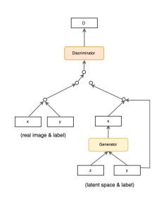
the idea is to impose some conditioning factor such as a label to be able impose generation in a more controlled manner.

InfoGAN

Creative design of GAN in order to address slightly different task. the main idea of InfoGAN is that we use the GAN to understand if there are some groups inside the data.

Can i have a GAN to understand if the data are in some classes? here the label are treated as latent factor and doing in a way that are consistent with the real label (MNIST eg). The latent code will be correlated with some group information, we impose the network to learn the latent code but also to learn information that are semantically related to the classes in the dataset.

Wasserstein GAN

For improving the gradient descent one measure improvement is this called Wasserstein GAIN whe a different difference measure is used. Different cost function, better gradients, more stable training.

More important the objective function value is more meaningfully related to quality of the generator output (test loss related to the quality of the image).

LSGAN

We replace the objective function with a different, instead the log loss with least square losses for generator and discriminator allowing more stable and robust trainings. Better quality images and more robust to mode collapse.

Image2Image translation

instead of using random noise can we use an image from a different domain? instead of random noise we have a transformation networks.

What if i feed a segmentation mask, can i have a GAN that produces a realistic images that comply this segmentation? from landscape can i have a GAN that produces a map?

Pix2Pix network

The network is considering pair of images (as in sequence) from example a scene and a corresponding segmentation and the goal is to train the discriminator accordingly to classify if the pairs of scenes were true or not.

Instead of having random noise i have a transformation network that is still trained in an adversarial network, the generator will be translate into an image of the output domain and the discriminator will try to understand which are the mode (from segmentation it generate the real image and the discriminator have to distinguish between the generated and real).

This required a paired images but this is a limiting factor.

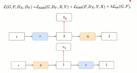
CycleGAN

complete unpaired image to image translation, the goal is to learn a transformation across domain. We do not have paired information we have a lot of images not paired.

The idea is that here we have two generator and two discriminator that operate in their own distribution and learn a mapping to translate their distribution to the others.

it is a GAN that operate in two directions, i have a generator a discriminator and i also have a reconstruction network. I want to translate the images of real photography to van gogh paintings.

From real image the nn learn how to generate van gogh images (compare the generated van gogh with real van gogh) what is new is that another network that will try to reconstruct the original image.

This is done in two directions and the two networks will share the parameters:

Text-To-Image synthesis

Can i condition the generator not only with visual information but also with text information? if together with noise i add some text information and impose the network to generate images that are associated to this text (the discriminator will do the same but with text description).

I’m expanding the conditional gan with text instead of only labels.

GAN Summary

• Gans do not consider an explicit density function
• A game-theoretic approach is used;
• the models learn how to generate sample from training data trough a two-player game (introducing the discriminator).

the main problem is that is tricky and unstable to train and we do not have a proper way to check the results.

Non Probabilistic Approach

Autoencoders

In some situation unsupervised learning are used to compress data, here i want to learn some non-linear transformation into a lower dimension while keeping the most important features.

Autoencoders are very old, they were a technique for training a backbone for supervised learning task. The core idea is to encode information, compress information automatically. The compression is because i have a first network that compress the information and then a decoder that mirror the structure of the encoder and gets back to the original image. The best compact representation of the data is the one that allow to reconstruct the image.

autoencoders is an unsupervised approach for learning a lower-dimensional feature representation from unlabeled training data.

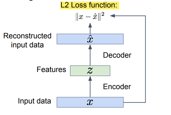
the dimension of $z$ usually is smaller than $x$ since only the relevant features are kept and the noise is suppressed. We train such that features can be used to reconstruct original data “Autoencoding” - encoding itself.

for implementing the encoders we can use some linear layer plus some non linear activation functions. Originally the used Linear Layers + sigmoid functions then start using CNN architectures for encoding the image into the latent feature and deconvolutional layer for recreating the image.

At the beginning autoencoders were use to initialize a supervised model, basically they were used as feature extractor.

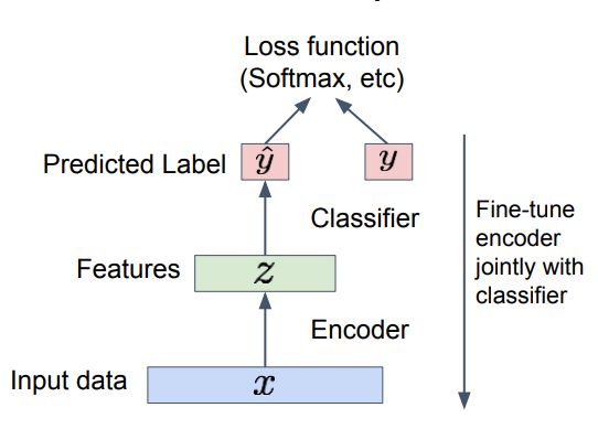
Similar to GAN once the training is over we discard the reconstructor and use only the encoder model.

One popular variation is the denoising autoencoders, to force the auto-encoder to learn useful features is adding random noise to its inputs and making it recover the original noise-free data.

Explicit density model

AutoRegressive models

the GAN does not try to learn a probabilistic model but instead the idea of auto-regressive model is to explicitly model the likelihood of each image and since each image is composed by pixel we would like to decompose the likelihood of an image into the product of the likelihood of each pixels (if i observe the pixel in position i it depends to others pixel, called context).

Use chain rule to decompose likelihood of an image x into product of 1D distributions where the likelihood of image $x$ is the product of several probability condition, in particular the probability of pixel $I$ given the previous (called context).

$p_{\theta}(x)= \prod_{i=1}^{n} p(x_{i}| x_{1}, … , x_{i-1})$

This approach turns the modeling problem into a sequence problem wherein the next pixel value is determined by all the previously generated pixel values. The problem of generation is addressed as problem of learning a sequence (sequence of pixel given the context).

Which is the neural net that is the best for express this probability distributions, this require the decision of the network (recurrent or convnet) and the decision of the context.

The main problems with this approach is that we have to define the ordering of previous pixels and most important since they predict one pixel at the time they are very slow.

PixelRNN

First approach tried was to use the LSTM for capturing the context, the models start from the corner and the dependencies are captured using a two-dimensional LSTM; Here we have to also consider the channel dependencies. The image is generated pixel by pixel.

For solving the problem of conserving spatial information is using the diagonal BiLSTM in order to capturing the most meaningful context as possible. Diagonal because i need the spatial context not only temporal. More over the image is a tensor not a matrix so it was necessary to create dependencies among the different channels.

The main advantage of this approach is that using an explicit density model we have a simple way to compare methods and results since we can compare directly the resulting distribution while the main drawback is that the are very slow (one pixel at the time) and the quality is low.

PixelCNN

they tried to address the slow sequential generation using a CNN rather than a recurrent nn.

Still generate one pixel at the time starting from the cornel but in this case we use a convolutional nn rather than a RNN. Dependency on previous pixels now modeled using a CNN over context region. I can still address generation the pixel according to the context trough a usage of a mask.

they still generate one pixel at the time but for the training phase we can parallelize the operation but at test time not.

At each point we sill predicting a vector [0,255] representing the probabilities of the pixel value:

Training is faster than PixelRNN (can parallelize convolutions since context region values known from training images) but at the test time it is still slow since it has to compute one pixel at the time.

a little variation of pixel CNN is using multi-scale context where we do not use all the previous pixels but just a grid of them. This can be done with pixel cnn using the delation kernel.

AutoRegressive advantages

Pros:

• Can explicitly compute likelihood p(x)
• Explicit likelihood of training data gives good evaluation metric.
• Good samples

the main disadvantages regard the computation time and the assumptions made to capture the context.

Variation AutoEncoders (VAE)

Can i take autoencoders and move to the probabilistic word?

PixelCNNs define tractable density function, optimize likelihood of training data:

$p_{\theta}(x)= \prod_{i=1}^{n} p(x_{i}| x_{1}, … , x_{i-1})$

VAEs define in tractable density function with latent $z$:

$p_{\theta}(x) = \int p_{\theta}(z) p_{\theta}(x|z) dz$

where $p_{\theta}(z)$ is the simple gaussian prior distribution of the latent features while $p_{\theta}(x|z)$ is the decoder nn. they are defining the probabilities by marginalizing such a latent space.

Cannot optimize directly, derive and optimize lower bound on likelihood instead; VAEs are combination of autoencoders with Variational approximation and variational lower bound.

Autoencoder that operate on latent features and pas hem into a probabilistic view that allow to optimize the likelihood function.

in autoencoders there is nothing that force the latent space to be in a good probability distribution space, the main idea is to rephrase autoencoders with a probabilistic spin.

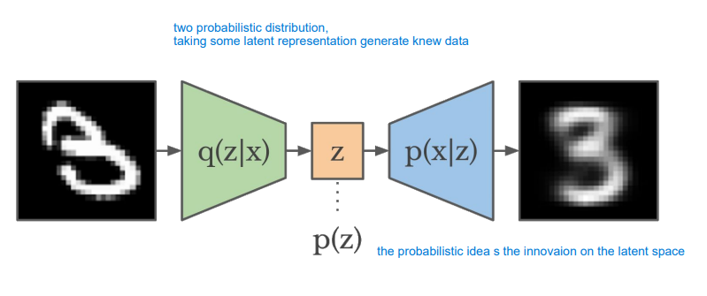
We will have two models: a function represented by the encoder that produces the latent feature representation given the image $z|x$ and then we have the decoder that emulate the function $x$ given $z$. And we use the $p(z)$ a simple gaussian probability distribution, so the latent space will be forced to be similar to another distribution (such as a gaussian distribution). The difference is in this core probabilistic approach to the latent space.

we want to give to our latent feature a probabilistic fashion and so we want the ability to sample from a probability distribution associated with our latent space.

$z$ is the latent factor used to generate the images back, i’m interested to estimate the optimal parameters according to the maximum likelihood, in order to do this i need to define some choices (the prior distribution for $z$ is a gaussian).

The main problem is that when learning the parameters to maximize the likelihood of the training data the optimization function is intractable (cannot compute $p(x|z)$ for every $z$). The object to maximize is intractable.

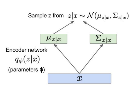
at the end the main intuition is that i have a first neural network that model the first conditional distribution $p_{\theta} (x|z)$ and then i will have another neural network that model the mirror conditional distribution $q_{\phi} (z|x)$.

This means that the encoder network is a nn that learn how to predict the mean and the covariant of the first distribution. while the decoder will be another neural network that produce the mean and the covariance for the second conditional distribution (since we have to sample we have to implement the reparametrization tricks for gradient descent).

we then sample z with the mean and covariance estimated and reconstruct x from z with the mean anf covariance estimated trough the decoder.

Solution: In addition to decoder network modeling $p_{\theta} (x|z)$, define additional encoder network $q_{\phi} (z|x)$ that approximates $p_{\theta} (z|x)$. This allows us to derive a lower bound on the data likelihood that is tractable, which we can optimize.

$log p_{theta}(x^{(i)}) = E_{z} [log p_{\theta} (x^{(i)}|z)] - D_{KL} (q_{\phi}(x^{(i)}|z)|| p_{\theta}(z)) + D_{KL} (q_{\phi}(x^{(i)}|z)|| p_{\theta}(z|x^{(i)})) $

i want to maximize the llikelhood of my training point and at the end this likelihood is intractable, is the sum of three term and one of them in not possible to compute but since it is a kullbach divergence we know that is greater than zero.

where $log p_{\theta} (x^{(i)}|z)$ is the reconstruct of the input data somehow i want my nn to fit well the data (over the parameter of the decoder), the second KullbachLeiber divergence $- D_{KL} (q_{\phi}(x^{(i)}|z)|| p_{\theta}(z))$ is referred to make approximate posterior distribution close to the prior, it force the latent distribution similar to prior distribution (gaussian) and the last term is the intractable part that is always > 0. The loss is called variational lower bound “ELBO”. Here the two models go in the same direction, there is no adversarial fashion.

this training involve sampling, to be able to do this we use the reparametrization trick.

if i use normal autoencoders i will have some discontinuity in the latent space; how do i ensure if i taken a latent code i produce a meaningful reconstructed image? This is indeed real in VAE because the KullbachLeiber term push the distribution to be similar to a prior. I will have closer point in the latent space that are similar to a particular digit and i do not have discontinuity moving inside the latent space, if we interpolate from the latent space representing ‘1’ and ‘2’ in the middle i’ll have something that seems to both while in normal autoencoders could not be the case. VAE allow to move smoothly in the latent feature producing different concepts.

Once the model is trained we can use the decoder network to sample $z$ from a prior distribution and generating new images and we can think as the dimension of $z$ as feature of the images itself (like head pose for $z_{1}$ or degree of similarity $z_{2}$). Since we are learning a certain priori it means that we are learning independent latent variable that will be encoded with different degree of variation in the data.

to sum up: VAE are a Probabilistic spin to traditional autoencoders in which a intractable density is defined and is derive and optimized indirectly trough a lower bound.

with VAE we are able to generate complete new image by perturbating the latent feature space $z$. vae are a probabilistic twist on autoencoders, sample from the mean and sd to compute the latent space. we break down the latent space z into a mean vector and a standard deviation, the goal of the encoder is to output a mean and sd that correspond to the distribution of $z$ vector introducing an element of stocasticity.

both encoder and decoder are probabilistic in nature, the encoder wll try to infer the probability distribution of the latent space respect to the data $q_{\phi}(z|x)$ while the decoder is trying to infer a new probability distribution of the input given the latent distribution $p_{\theta}(x|z)$.

The loss is given by

$L(\phi, \theta, x) = reconstruction\ loss + regularization\ term$

where the reconstruction loss is given by typically L2 norm between the input image and the reconstructed image. while the regularization term: $D(q_{\phi}(z|x) || p(z))$. The term $q_{\phi}(z|x)$ is the computation that our encoder try to learn (distribution of latent space given the data $x$) and what we do regularizing this network is to place a prior distribution (it means some initial hypothesis about the real distribution could look likes) and will help the network to create a structure that roughly follow this prior distribution to be. This prior is usually a gaussian distribution meaning that is center in mean with 0 and variance of 1, this means in practice to place the latent vectors in the center of this latent space. the kl divergence is a measure of how far are two distributions.

Using a prior as a gaussian distribution allow us to have some desired properties:

1. Continuity: if two points are similar in the latent space means that they will be similar after decoding.
2. Completeness: when we sample from the latent space we want to obtain always meaningful content after decoding.

how in practice we can train this network, end to end? by imposing this probabilistic we introduce stochasticity, during backprop we cannot propagate back since it is stochastic. The idea to solve this it to reparametrizing this sampling layer. The core idea is to more the stochasticity away frm the mean and sigma that we want to train basically keeping a fixed $\mu$ and fixed $\sigma$ and scale them bny a random constant.

Vae with this notion of distribution over latent variable we can sample and perturb and tune the variable of feature keeping all the rest fixed and the output image change in the features (as head pose).

Conditional

If we have labels we can use the conditional information and the loss function will change minimal.

Conditional vae introduce the usage of the labels (or inputs in which we can condition the process) in the process, in this case twe just replace $p(x|z)$ with $p(x|z,y)$ and $q(x|z)$ with $q(x|z,y)$ and we go trough the same KL divergence procedure to the the same lower bound.

The VAE was the first technique to perform the task of attribute-conditionated image generation, so they tried to embed a caption in an appropriate space and then enabling such a generation creating images according to the description.

Basically we are modifying the latent feature with some kind of knowledge derived from the label.

VAE vs GAN

some researcher to put together VAE and GAN and to create this combination model. in VAE is easy to find $z$ and we work addressing explicitly the likelihood but the problem is that the output blurry images. the VAE-GAN is to put together the best of both work, we will regenerator the images and then this image will be passed trough a real image to a discriminator.

Final comparison

there are three family of models:

1. Autoregressive model: that allow a simple and stable training, they directly operate on the likelihood of the data. However they are highly inefficient (and do not provide any latent space)

2. GAN: produces the sharpest images but the main difficulties is the unstable training dynamics.

3. VAE: they are the best in order to map the data into a latent space (well organized) but tends to have blurry outputs.