 Learning
theory - Conv Nets
Convolutional Neural Network
When our data are in a particular form like images or sequences Neural network outperform the traditional shallow models.
they are inspired by mammalian visual cortex; the brain is structured in different sections to recognize objects and create a body reaction, each section has a specific task to solve.
- The first layers are used to detect edges, corners and simple shapes.
- Based on these detections more complex shapes can be recognized.
- Only at the last layers (AIT) real object representations are produced.
The visual cortex contains a complex arrangement of cells, which are sensitive to small sub-regions of the visual field, called a receptive field.
Two basic cell types:
-
Simple cells respond maximally to specific edge-like patterns within their receptive field.
-
Complex cells have larger receptive fields and are locally invariant to the exact position of the pattern.
in the 1962 Hubel & Wiesel studies suggested a hierarchy of feature detectors in the visual cortex, basically the first layers find easy patterns as edges and lines while higher layers merge this feature into more complex ones.
Convolutional networks, also known as convolutional neural networks, or CNNs, are a specialized kind of neural network for processing data that has a known grid-like topology. The name ‘convolutional neural network’ indicates that the network employs a mathematical operation called convolution. Convolution is a specialized kind of linear operation. Convolutional networks are simply neural networks that use convolution in place of general matrix multiplication in at least one of their layers.
CNN Architecture
Convolutional Neural Networks are multi-layer neural networks with local connectivity: neurons in a layer are only connected to a small region of the layer before it. They share weight parameters across spatial positions allowing Learning shift-invariant filter kernels and to reduce the number of parameters.
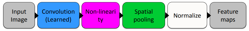
CNN are neural network with specialized connectivity structure they stack multiple layers of feature extractors where the low-level layers extract local features while high level layers extract and learn more complex and global patterns. There are a few distinct types of operations:
- Convolution
- Non-linearity
- Pooling
the convolutional layers consists of a set of filters, each filter is convolved across the dimensions of the input data, producing a multi-dimensional feature map.
Convolution
Convolutional networks are simply neural networks that use convolution in place of general matrix multiplication in at least one of their layers.
$S(i,j) = (I*K)(i,j) = \sum_{m} \sum_{n} I(m,n) K (i-m, j-n)$
$s(t) = \int x(a) w(t-a) da$
Convolution is an operation on two functions of a real-valued argument, The first function $x$ is referred to as the input, the second function $w$ is referred to as the kernel; The output $s$ is also a function. In deep learning we are interested in matrix and in 2D images for filtering operation.
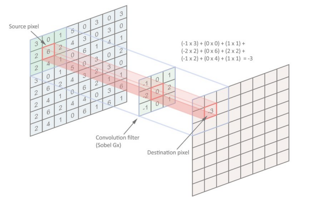
Convolution is a general purpose filtering operation for images where a kernel matrix is applied to an image. It works by determining the value of a central pixel by adding the weighted values of all its neighbors together. the first approach was to design already made kernels, so using handcrafted kernels but then using deep neural network we let the nn learn the best kernels.
Differently sized kernels containing different patterns of numbers produce different results. The size of a kernel is arbitrary (3x3, 5,5; bigger means more aggressive). Convolutions can be used to smooth, sharpen, enhance, the approach in the past was to use pre-made kernels.
Using convnet we are able to preserve the spatial structure in the input; the idea is that each neuron of our nn is going to see only a patches of data. Pixels that are close to each other there is highly probability that they share information. These patches are called kernel and basically we slide the kernel all over the images (se the feature learned all across the image).
we have a feature map that denotes at any single location the straight to detecting that filter at that location in the input pixel. if the features is found the sum f the feature map will be higher otherwise low. Changing the weights into the kernel we can represent complete different features.
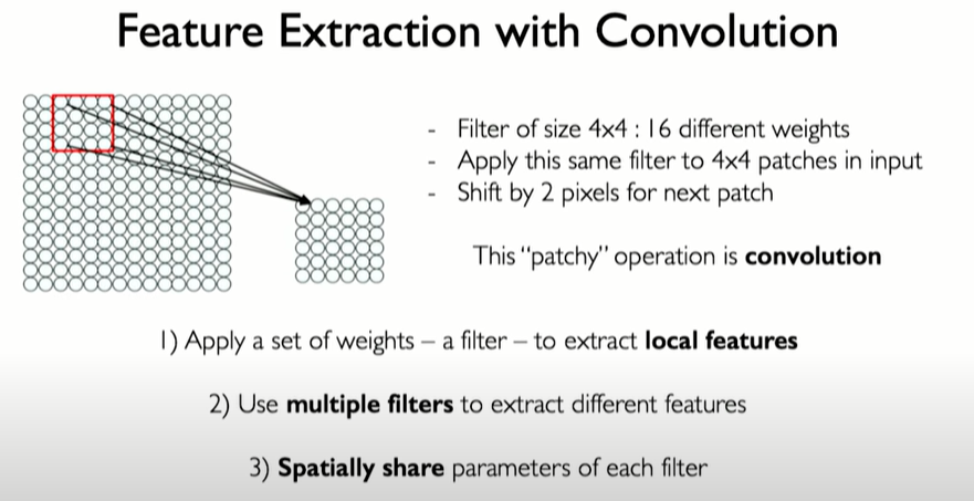
Within a single convolutional layer we can have multiple filters, the output of each layer now is a volume of images. One image corresponding to each filter that is learned.
recap: given an input matrix and given a kernel (3x3 matrix) then the results of the convolution is another matrix and each element is composed by the considering all the inputs multiplied by the kernel summing them up; then we slight the filter and do the same operation over the neighbor source pixel.
Convolution Params
Main conv parameters:
-
Stride: moving the kernel by $n$ pixel each times (equal to 1 means that the kernel slice by one cell), Input size $N$, kernel with receptive field $K$, stride $S$ $Output \ size= (N-K)/S + 1$.
-
Padding: Often, we want the output of a convolution to have the same size as the input. Solution: use zero padding, so add a border filled with zeros. If we have as input a tensor $W_{1} × H_{1} × D_{1}$ , the filter size is $K$ and the stride is $S$. we get that:
$W_{2} = (W_{1} - K) / S +1$ $H_{2} = (H_{1} - K) / S +1$
Non-linearity
In the second stage, each linear activation is run through a nonlinear activation function, such as the rectified linear activation function.This stage is sometimes called the detector stage (Pixel levels of non-linearity, the negative values represent .
Pooling
In the third stage, we use a pooling function to modify the output of the layer further. A pooling function replaces the output of the net at a certain location with a summary statistic of the nearby outputs. For example, the max pooling operation reports the maximum output within a rectangular neighborhood.
- Dimensionality reduction
- Invariance to transformations of translation
In all cases, pooling helps to make the representation approximately invariant to small translations of the input. Invariance to translation means that if we translate the input by a small amount, the values of most of the pooled outputs do not change. Invariance to local translation can be a useful property if we care more about whether some feature is present than exactly where it is. For example, when determining whether an image contains a face, we need not know the location of the eyes with pixel-perfect accuracy, we just need to know that there is an eye on the left side of the face and an eye on the right side of the face.
Engineered vs learned features
Typically in ML was tradition to handcraft the kernel for the feature extractors, the revolution of conv net is that we let the nn learn what are the best kernel for our goals.
The manual feature extraction is problematic for many reasons such as viewpoint variation, illumination conditions, scale condition, scale variation, occlusion, intra class variation and many others. In convolutional neural network this patterns are learned by the nn itself. Using convnet we can learn a hierarchy of features directly the data instead of hand engineering them.
visual representation of conv operation
…. To a compute an images is just a collection of numbers, in particular a 1 or 3 dimensional matrix.
Evolution of Convnets
LeNet-5
LeNet-5 was the first “famous” CNN architecture, which was developed by LeCun et al. (1998, for recognition of handwritten digits. LeCun and his fellow researchers were working on CNN models for a decade to come up with an efficient architecture.
It was a very shallow CNN by modern regards and had only about 60,000 parameters to train for an input image of dimensions 32x32x1.
LeNet5(
  (feature_extractor): Sequential(
    (0): Conv2d(1, 6, kernel_size=(5, 5), stride=(1, 1))
    (1): Tanh()
    (2): AvgPool2d(kernel_size=2, stride=2, padding=0)
    (3): Conv2d(6, 16, kernel_size=(5, 5), stride=(1, 1))
    (4): Tanh()
    (5): AvgPool2d(kernel_size=2, stride=2, padding=0)
    (6): Conv2d(16, 120, kernel_size=(5, 5), stride=(1, 1))
    (7): Tanh()
  )
  (classifier): Sequential(
    (0): Linear(in_features=120, out_features=84, bias=True)
    (1): Tanh()
    (2): Linear(in_features=84, out_features=10, bias=True)
  )
)
AlexNet
Similar framework to LeNet but:
- Bigger model (7 hidden layers, 650,000 units, 60kk params)
- More data (ImageNet challenge)
- GPU implementation
AlexNet(
  (features): Sequential(
    (0): Conv2d(3, 64, kernel_size=(11, 11), stride=(4, 4), padding=(2, 2))
    (1): ReLU(inplace=True)
    (2): MaxPool2d(kernel_size=3, stride=2, padding=0, dilation=1, ceil_mode=False)
    (3): Conv2d(64, 192, kernel_size=(5, 5), stride=(1, 1), padding=(2, 2))
    (4): ReLU(inplace=True)
    (5): MaxPool2d(kernel_size=3, stride=2, padding=0, dilation=1, ceil_mode=False)
    (6): Conv2d(192, 384, kernel_size=(3, 3), stride=(1, 1), padding=(1, 1))
    (7): ReLU(inplace=True)
    (8): Conv2d(384, 256, kernel_size=(3, 3), stride=(1, 1), padding=(1, 1))
    (9): ReLU(inplace=True)
    (10): Conv2d(256, 256, kernel_size=(3, 3), stride=(1, 1), padding=(1, 1))
    (11): ReLU(inplace=True)
    (12): MaxPool2d(kernel_size=3, stride=2, padding=0, dilation=1, ceil_mode=False)
  )
  (avgpool): AdaptiveAvgPool2d(output_size=(6, 6))
  (classifier): Sequential(
    (0): Dropout(p=0.5, inplace=False)
    (1): Linear(in_features=9216, out_features=4096, bias=True)
    (2): ReLU(inplace=True)
    (3): Dropout(p=0.5, inplace=False)
    (4): Linear(in_features=4096, out_features=4096, bias=True)
    (5): ReLU(inplace=True)
    (6): Linear(in_features=4096, out_features=n_of_classes, bias=True)
  )
)
Consists of eight layers — Five convolutional layers and three fully connected layers. Uses ReLu (Rectified Linear Units) in place of the tanh function, giving a 6x times faster dataset than a CNN using tanh; The problems with overfitting increased with the use of 60 million parameters. This was taken care of by dropping out neurons with a predetermined probability (say 50%) and data augmentation.
AlexNet gives 4096 dimensional features for each image. AlexNet discovers general features of the input space serving multiple tasks (now true for other architectures as well).
in the same period of time there were a large debate if the model trained could be used in others context, they understood that using large pretrained models improve drastically the performance.
ZFNet
ZFNet was an improved version of AlexNet, proposed by Zeiler et al. (2013). The main reason that ZFNet became widely popular because it was accompanied by a better understanding of how CNNs work internally.
in the ILSVRC 2013 the challenge The challenge was won by a network similar to AlexNet changing a little the architectures and using less aggressive kernels.
Understanding CNN
But with ZFNet, came a novel visualization technique through a deconvolutional network. Deconvolution can be defined as the reconstruction of any convoluted features into a human-comprehensible visual form. Hence, this helped researchers to know what they were exactly doing.
Difficult to understand internals of CNNs, Zeiler & Fergus in 2013 tried to exploit this problem aiming to interpret activity in intermediate layers. the core idea was to recreate the image back from the features using some deconvolutional network.
These experiments demonstrate what was supposed before for example that the features are learned hierarchically trough the layers.
Occlusions Experiments
Zeiler and Fergus also used feature visualizations to see if network really identified the object or depended on context Occluding images at different locations and visualize feature activations and classifier confidence.
Class Model Visualization
trying to understand the image that have the maximum score for the given class (so the image that best represent a class representation for the model) by simply optimizing the generator model following.
GoogLeNet
GoogLeNet was proposed by Szegedy et al. in 2015 as the initial version of the Inception; this model put forward state of the art image classification and detection in the ImageNet Large-Scale Visual Recognition Challenge 2014 (ILSVRC14) and secured the first place in the competition.
The network is 22 layers deep (27 layers if pooling is included); a very deep model when compared to its predecessors but with less parameters; Gets rid of fully connected layers and used 1x1 convolutions to limit the number of channels.
VGG-16
VGG-16 was the next big breakthrough in the deep learning and computer vision domains, as it marked the beginning of very deep CNNs. Earlier, models like AlexNet used high dimensional filters in the initial layers, but VGG changed this and used 3x3 filters instead. This ConvNet developed by Simonyan and Zisserman (2015) became the best performing model at that time and fueled further research into deep CNNs.
t approximately had an overwhelming 138 million parameters to train which was more than at least twice the number of parameters in other models used then. Hence, it took weeks to train.
VGG(
  (features): Sequential(
    (0): Conv2d(3, 64, kernel_size=(3, 3), stride=(1, 1), padding=(1, 1))
    (1): ReLU(inplace=True)
    (2): Conv2d(64, 64, kernel_size=(3, 3), stride=(1, 1), padding=(1, 1))
    (3): ReLU(inplace=True)
    (4): MaxPool2d(kernel_size=2, stride=2, padding=0, dilation=1, ceil_mode=False)
    (5): Conv2d(64, 128, kernel_size=(3, 3), stride=(1, 1), padding=(1, 1))
    (6): ReLU(inplace=True)
    (7): Conv2d(128, 128, kernel_size=(3, 3), stride=(1, 1), padding=(1, 1))
    (8): ReLU(inplace=True)
    (9): MaxPool2d(kernel_size=2, stride=2, padding=0, dilation=1, ceil_mode=False)
    (10): Conv2d(128, 256, kernel_size=(3, 3), stride=(1, 1), padding=(1, 1))
    (11): ReLU(inplace=True)
    (12): Conv2d(256, 256, kernel_size=(3, 3), stride=(1, 1), padding=(1, 1))
    (13): ReLU(inplace=True)
    (14): Conv2d(256, 256, kernel_size=(3, 3), stride=(1, 1), padding=(1, 1))
    (15): ReLU(inplace=True)
    (16): MaxPool2d(kernel_size=2, stride=2, padding=0, dilation=1, ceil_mode=False)
    (17): Conv2d(256, 512, kernel_size=(3, 3), stride=(1, 1), padding=(1, 1))
    (18): ReLU(inplace=True)
    (19): Conv2d(512, 512, kernel_size=(3, 3), stride=(1, 1), padding=(1, 1))
    (20): ReLU(inplace=True)
    (21): Conv2d(512, 512, kernel_size=(3, 3), stride=(1, 1), padding=(1, 1))
    (22): ReLU(inplace=True)
    (23): MaxPool2d(kernel_size=2, stride=2, padding=0, dilation=1, ceil_mode=False)
    (24): Conv2d(512, 512, kernel_size=(3, 3), stride=(1, 1), padding=(1, 1))
    (25): ReLU(inplace=True)
    (26): Conv2d(512, 512, kernel_size=(3, 3), stride=(1, 1), padding=(1, 1))
    (27): ReLU(inplace=True)
    (28): Conv2d(512, 512, kernel_size=(3, 3), stride=(1, 1), padding=(1, 1))
    (29): ReLU(inplace=True)
    (30): MaxPool2d(kernel_size=2, stride=2, padding=0, dilation=1, ceil_mode=False)
  )
  (avgpool): AdaptiveAvgPool2d(output_size=(7, 7))
  (classifier): Sequential(
    (0): Linear(in_features=25088, out_features=4096, bias=True)
    (1): ReLU(inplace=True)
    (2): Dropout(p=0.5, inplace=False)
    (3): Linear(in_features=4096, out_features=4096, bias=True)
    (4): ReLU(inplace=True)
    (5): Dropout(p=0.5, inplace=False)
    (6): Linear(in_features=4096, out_features=1000, bias=True)
  )
)
ResNet - 2016
ResNet was put forward by He et al. in 2015, a model that could employ hundreds to thousands of layers whilst providing compelling performance. The problem with deep Neural Networks was of the vanishing gradient, repeated multiplication as the network goes deeper, thereby resulting in an infinitely small gradient.
ResNet looks to introduce shortcut connections by skipping one or more layers. Here, these perform identity mappings, with outputs added to those of the stacked layers.
Key features:
- Only ~2M parameters (using many small kernels, 1x1, 3x3)
- Adds identity bypass: If layer will not be needed it can simply be ignored; it will just forward input as output
- Reduction of internal covariance shift with Batch Normalization
Using residual connections they’ve been able to solve the vanishing gradients problem and going very deep. One reason why ResNet works is also that it can be seen as implicitly ensembling shallower networks.
ResNet(
  (conv1): Conv2d(3, 64, kernel_size=(7, 7), stride=(2, 2), padding=(3, 3))
  (bn1): BatchNorm2d(64, eps=1e-05, momentum=0.1)
  (relu): ReLU(inplace=True)
  (maxpool): MaxPool2d(kernel_size=3, stride=2, padding=1, dilation=1)

  (layer1): Sequential(
    (0): BasicBlock(
      (conv1): Conv2d(64, 64, kernel_size=(3, 3), stride=(1, 1), padding=(1, 1))
      (bn1): BatchNorm2d(64, eps=1e-05, momentum=0.1)
      (relu): ReLU(inplace=True)
      (conv2): Conv2d(64, 64, kernel_size=(3, 3), stride=(1, 1), padding=(1, 1))
      (bn2): BatchNorm2d(64, eps=1e-05, momentum=0.1)
    )
    (1): BasicBlock(
      (conv1): Conv2d(64, 64, kernel_size=(3, 3), stride=(1, 1), padding=(1, 1))
      (bn1): BatchNorm2d(64, eps=1e-05, momentum=0.1)
      (relu): ReLU(inplace=True)
      (conv2): Conv2d(64, 64, kernel_size=(3, 3), stride=(1, 1), padding=(1, 1))
      (bn2): BatchNorm2d(64, eps=1e-05, momentum=0.1)
    )
  )
  (layer2)
  (layer3)
  (layer4)
  (avgpool): AdaptiveAvgPool2d(output_size=(1, 1))
  (fc): Linear(in_features=512, out_features=1000, bias=True)
)
Wide ResNet
Use ResNet basic block with more feature maps; Investigated relationship between width and depth to find a good trade-off.
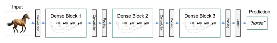
DenseNet
Every layer is connected to all other layers. For each layer, the feature maps of all preceding layers are used as inputs, and its own feature maps are used as inputs into all subsequent layers.
Suggestions
There are tons of new architectures that look very different; Upon closer inspection, most of them are reapplying well established principles.
- Universal principles seem to be having shorter sub paths through the networks
- Identity propagation (Residuals, Dense Blocks) seem to make training easier
- Feature reuse is definitely a good idea.
- Reduce filter sizes (except possibly at the lowest layer), factorize filters aggressively
- Use 1x1 convolutions to reduce and expand the number of feature maps judiciously
- Use skip connections and/or create multiple paths through the network
R-CNN use some algorithm (heuristics) to found possible boxes (then shrinks to a specific size) and classified it. separate jobs.
faster r.cnn to tackle this issue, image input directly into convolutional feature extractor. We can as input the entire image and the first think is that the conv has a proposal region where it may be interesting regions (completely learned).
CNN Applications
Object Detection
Simultaneous Classification and Regression, the output is a bounding boxes ($x_{1}, y_{1}, x_{2}, y_{2}$) and the labels for each object in the image.
The main challenge around this task is the PASCAL VOC Challenge which was include predict the bounding box and the labels of each object from 20 target classes. At the very first time almost all possible bounding box were tried.
in this context we deal with a multi task loss combining the classification loss with the bounding-box regression loss.
Selective Search (Region proposal)
A possible improvement is to use an external procedure that may produce a useful areas to search in rather than all possible combinations. This first attempt was done using the selective search (which looks for local patterns of the picture like pattern brightness and similar).
the goal of the selective search is to detect objects at any scale, this was done using a hierarchical algorithms moreover it consider multiple grouping criteria like the differences in color, texture, brightness and others.
The core idea is to use bottom-up grouping of image regions to generate a hierarchy of small to large regions:
- Generate initial sub-segmentation (start small objects and then aggregate them into larger objects).
- Recursively combine similar regions into larger ones (based on the feature describe above)
- Use the generated regions to produce candidate object locations;
the results is a set of possible candidate object locations where the conv net will try to classify the object.
This process was not completely bad but the main problem was that we do not learn the best possible candidates but instead we use some heuristic to produce the region proposal.
Once they have understood that the features learned by a model are useful also in similar tasks they try to use pretrained conv net also for this task.
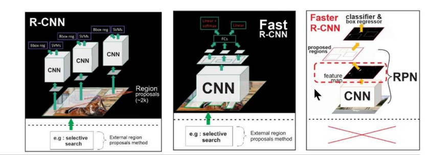
R-CNN: Regions with CNN features
To bypass the problem of selecting a huge number of regions, Ross Girshick et al. proposed a method where we use selective search to extract just 2000 regions from the image and he called them region proposals. These 2000 region proposals are generated using the selective search algorithm.
These 2000 candidate region proposals are warped into a square and fed into a convolutional neural network that produces a 4096-dimensional feature vector as output. The CNN acts as a feature extractor and the output dense layer consists of the features extracted from the image and the extracted features are fed into an SVM to classify the presence of the object within that candidate region proposal.
the main problem with R-CNN:
- It still takes a huge amount of time to train the network as you would have to classify 2000 region proposals per image.
- you need to crop and scale all the proposal into a specific size images.
- It cannot be implemented real time as it takes around 47 seconds for each test image.
- The selective search algorithm is a fixed algorithm. Therefore, no learning is happening at that stage. This could lead to the generation of bad candidate region proposals.
Fast R-CNN
The same author of the previous paper(R-CNN) solved some of the drawbacks of R-CNN to build a faster object detection algorithm and it was called Fast R-CNN. The approach is similar to the R-CNN algorithm. But, instead of feeding the region proposals to the CNN, we feed the input image to the CNN to generate a convolutional feature map.
From the convolutional feature map, we identify the region of proposals and warp them into squares and by using a RoI pooling layer we reshape them into a fixed size so that it can be fed into a fully connected layer.
(RoI (Region of Interest) Pooling: shares the forward pass of a CNN for an image across its selected subregions, it allow multiple dimension and reshape different map to a feature representation that is equal).
The reason “Fast R-CNN” is faster than R-CNN is because you don’t have to feed 2000 region proposals to the convolutional neural network every time. Instead, the convolution operation is done only once per image and a feature map is generated from it. the proposal are generated once the feature map is extracted and is upon of it.
Faster R-CNN
Both of the above algorithms(R-CNN & Fast R-CNN) uses selective search to find out the region proposals. Selective search is a slow and time-consuming process affecting the performance of the network. Therefore, Shaoqing Ren et al. came up with an object detection algorithm that eliminates the selective search algorithm and lets the network learn the region proposals.
Similar to Fast R-CNN, the image is provided as an input to a convolutional network which provides a convolutional feature map. Instead of using selective search algorithm on the feature map to identify the region proposals, a separate network is used to predict the region proposals. The predicted region proposals are then reshaped using a RoI pooling layer which is then used to classify the image within the proposed region and predict the offset values for the bounding boxes.
-
First stage is the deep fully convolutional network that proposes regions called a Region Proposal Network(RPN). RPN module serves as the attention of the unified network
-
The second stage is the Fast R-CNN detector that extracts features using RoIPool from each candidate box and performs classification and bounding-box regression
YOLO: You Only Look Once
All of the previous object detection algorithms use regions to localize the object within the image. The network does not look at the complete image. Instead, parts of the image which have high probabilities of containing the object. YOLO or You Only Look Once is an object detection algorithm much different from the region based algorithms seen above. In YOLO a single convolutional network predicts the bounding boxes and the class probabilities for these boxes.
How YOLO works is that we take an image and split it into an SxS grid, within each of the grid we take m bounding boxes. For each of the bounding box, the network outputs a class probability and offset values for the bounding box. The bounding boxes having the class probability above a threshold value is selected and used to locate the object within the image.
Instance Segmentation
Instance segmentation assigns a label to each pixel of the image. It is used for tasks such as counting the number of objects; object detection and segmentation of all objects in the image.
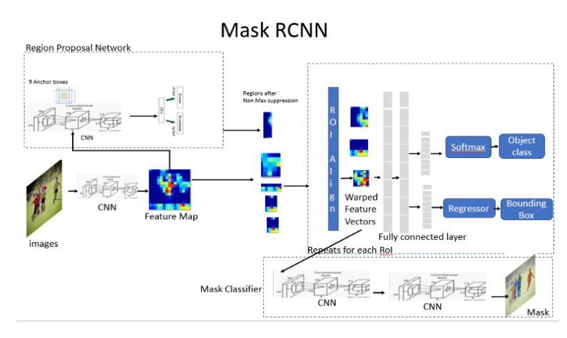
Mask R-CNN
Extend Faster R-CNN for pixel level segmentation. Mask R-CNN has an additional branch for predicting segmentation masks on each Region of Interest (RoI) in a pixel-to pixel manner it outputs three elements:
- For each candidate object, a class label and a bounding-box offset;
- Third output is the object mask
The RoI Align network outputs multiple bounding boxes rather than a single definite one and warp them into a fixed dimension. the Warped features are also fed into Mask classifier, which consists of two CNN’s to output a binary mask for each RoI. Mask Classifier allows the network to generate masks for every class without competition among classes
- CNN are flexible and can be successfully applied to object detection
- Learning features is essential not only for classification but also for detection
- The main challenge is speed and choice of the right architecture
- Modern architectures permit simultaneous detection and instance segmentation
Semantic Segmentation
in is used in many tasks as monocular depth estimation or self autonomous driving or medical imaging. the core idea is to reinterpret classification network as fully convolutional operation; doing these we still reduce the dimension of the input but keeping the convolutional layers and then we can expand back the convolution up-sapling the representation that have been learned.
For doing this operation we use pixel wise output loss.