 Learning

theory - Basic Nets components
- Estimation
- Deep Feed Forward Networks
- Cost functions and output units
- Gradient Descent
- How to learn weights? Backpropagation
- Optimizers
- Regularization
Estimation
Suppose we have N data points $X = {x_{1}, … , x_{N}}$ and suppose we know the probability distribution function that describes the data $p(y|x;\beta)$ and we want to determine the parameters $\beta$ that explain your data the best. We want to pick $\beta_{ML}$ (MaximumLikelihood), the $\beta$ s that explain the best our data; this plausibility of given data is measured by the log likelihood function $p(x, \beta)$.
$\beta_{ML} = arg max (\beta) \sum_{i=1}^{N} log (p_{model}(x^{i}; \beta))$
the procedure so consists of:
- Write the log likely hood function: $log p(x;\beta)$.
- Maximize: differentiate 1. w.r.t. $\beta$ and set the equation equal to 0.
- Solve for $\beta$ that satisfies the equation obtaining $\beta_{ML}$.
Most modern neural networks are trained using maximum likelihood. This means that the cost function is simply the negative log-likelihood, equivalently described as the cross-entropy between the training data and the model distribution.
The specific form of the cost function changes from model to model, depending on the specific form of $log p_{model}$. If we are dealing with probabilities we have to squeeze our distribution into a range of [0,1]. One recurring theme throughout neural network design is that the gradient of the cost function must be large and predictable enough to serve as a good guide for the learning algorithm. Functions that saturate (become very flat) undermine this objective because they make the gradient become very small. In many cases this happens because the activation functions used to produce the output of the hidden units or the output units saturate. The negative log-likelihood helps to avoid this problem for many models.
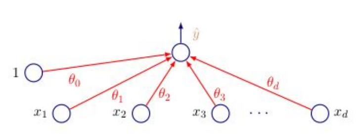
Considering the perceptron (When we are dealing with NN we apply the activation function to each neuron;) we can notice traduce the equation with a sigmoid activation as follow:
$p(y=1|x) = \frac{1}{1 + exp( - \beta_{0} - \beta^{T}x)}$
Having this in mind we can define the likelihood under the logistic model as follow:
$log(p(Y|X;\beta)) = \sum_{i=1}^{N} log p(y_{i} | x_{i}; \beta)$
This has no close formula but it converges but $log p(Y|X;\beta)$ is jointly concave in all component or equivalently, the error is convex so we can use gradient descent which is an iterative optimization algorithm, which finds the minimum of a differentiable function.
The largest difference between the linear models we have seen so far and neural networks is that the nonlinearity of a neural network causes most interesting loss functions to become non-convex. This means that neural networks are usually trained by using iterative, gradient-based optimizers that merely drive the cost function to a very low value, rather than the linear equation solvers used to train linear regression models or the convex optimization algorithms with global convergence guarantees used to train logistic regression
Deep Feed Forward Networks
The feedforward neural networks, or multilayer perceptrons(MLPs), are the quintessential deep learning models. The goal of a feedforward network is to approximate some function $f*$. A feedforward network defines a mapping $y=f(x;\beta)$ and learns the value of the parameters $\beta$ that result in the best function approximation.
Feedforward neural networks are called networks because they are typically represented by composing together many different functions. The model is associated with a directed acyclic graph (Information flow in function evaluation begins at input, flows through intermediate computations to produce the category) describing how the functions are composed together. the concatenation of non linear functions allow to learn very complex functions. For example, we might have three functions $f^{(1)}$ $f^{(2)}$ and $f^{(3)}$ connected in a chain, to form $f(x)=f^{(3)}(f^{(2)}(f^{(1)}(x)))$ where $f^{(1)}$ is the first layer and so on. These chain structures are the most commonly used structures of neural networks (the depth s the number of function that compose a NN).
In the training process we want to optimize $\beta$ to drive $f(x, \beta)$ closer to $f^{*}(x)$. The training examples specify directly what the output layer must do at each point $x$; it must produce a value that is close to $y$. The behavior of the other layers is not directly specified by the training data. The learning algorithm must decide how to use those layers to produce the desired output, but the training data do not say what each individual layer should do. Instead, the learning algorithm must decide how to use these layers to best implement an approximation of $f*$. Because the training data does not show the desired output for each of these layers, they are called hidden layers.
Feedforward networks overcome the limitations of linear models trough the nonlinear transformation, to do so we can apply the linear model not to $x$ itself but to a transformed input $\phi(x)$, where $\phi$ is a non linear transformation. the extension is obtained trough the following steps:
- Do non linear transformation $x \rightarrow \phi(x)$
- Apply linear model to $\phi(x)$
- $\phi(x)$ gives features or a representation for $x$
How to choose the representation $\phi(x)$
- Use a generic $\phi(x)$ (poor generalization for highly varying of $f^{*}$).
- Engineer $\phi(x)$.
- Learn $\phi(x)$ from the data.
Learn $\phi(x)$ from the data is the approach of neural network, they gives up on convexity; the main pros is that we learn some $\phi(x)$ representation that are the best features for our training set but at the same time we give up on convexity. The engineering effort now is not on the designing of some $\phi(x)$ but n the architecture of the model (how many layers, activations and so on). Differently from traditional ML loss functions become non-convex, different from convex optimization, no convergence guarantees.
Cost functions and output units
The engineering part regarding Neural network regard different elements such as:
- Cost function
- Form of output
- Activation functions
- Architecture (number of layers etc)
- Optimizer
Cost function
to understand how good is our nn we use the loss which is the discrepancy between the ground truth and the predicted values; it depends on the task that we are dealing with. The loss function is a function of the network weights.
Classification context
typically in classification context we use the Binary cross-entropy (single class) or the Categorical cross-entropy (multi class). Choice of output units is very important for the choice of the cost function.
the BCE (which is the log likelihood) is computed as follow:
$-\frac{1}{N} \sum_{i=1}^{N} y_{i} * log( p(y_{i})) + (1 - y_{i}) * log (1- p(y_{i})) $
while the Categorical Cross-Entropy:
$-\sum_{i=1}^{n} y_{i} * log(p(y_{i}))$
where $y_{i}$ is the ground truth [0,1] whe the log of the probability is the output of the model after going trough a soft-max activation functions.
Regression context
in the regression context we tend to use the MSE $L=(y-f(x))^{2}$ or the MAE $L=|y-f(x)|$ but we can use also more advance cost function as the Huber function which combines MSE and AE: like MSE for small errors, like AE otherwise.
Output units ?
Hidden units
the procedure is the following:
- Accept input $x$
- Compute affine transformation $z= w^{T} x + b$
- Apply element-wise non-linear function $g(z)$.
ReLU
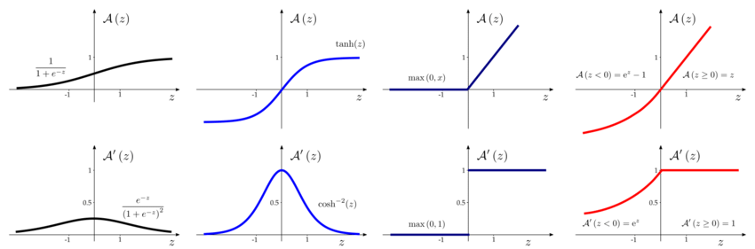
$g$ is always a non-linear function applied element-wise. The most used and important activation function is the Rectified Linear Units also called ReLU; it is very simple since it is just:
$g(z) = max {0,z}$
the derivative of the hidden units are very important since they tell if we are updating our parameter well or not, in the case of the ReLU the gradient is either zero when $z<0$ or 1 when $z>0$. It is similar to linear units since it is easy to optimize and give large and consistent gradients when active. a common practice is to initialize $b$ to a small positive values so that at the beginning all the neurons are used. The main positives aspects are that ReLU provide large and consistent gradients (does no saturate) and are efficient to optimize (converge faster than sigmoid) while the negatives aspect are that the output is nonzero centered and the units could “die” (no possibility to update when switch to inactive).
Generalized ReLU
after the ReLU many improvements have been tried all focusing around the concept of having a non-zero slope when $z<0$ like Leaky ReLU, Parametric ReLU, randomized ReLU. the main advantage of these neurons is that they do not kill neurons since they do no be stuck on zero.
Sigmoid units
in feed forward nn the activation function is typically ReLU but in other architectures as in conv NN we can still found different units such as the sigmoid:
$\sigma(x) = \frac{1}{1 + e^{-z}}$
Squashing type of non-linearity: pushes outputs to range [0,1]. Problem: Saturate across most of the domain, strongly sensitive only when z is closer to zero; Saturation makes gradient based learning difficult.
Tanh units
Similar to sigmoid but now the the output range will be [-1,1] and so the output will be zero centered. The derivative of sigmoid and tangent are derived from the original function itself and are easy to implement.
Gradient Descent
let’s try to find the best intercept and slope for a simple linear regression using gradient descent.
- Start only from the intercept (slope given) the first thing we do is pick a random value for intercept (initial guess), we compute the loss and we keep track of the results. With gradient descent we perform big step when we are far from the optimal solution and smaller steps when we are close to it. Gradient descent identifies the optimal value by taking bug steps when it is far away and small steps when it is close.
Starting from intercept = 0, we compute the cost and we can create basically an equation:
$MSE = (w_{1} - (intercept + b_{1} * h_{1})^{2}) + (w_{2} - (intercept + b_{1} * h_{2})^{2})$
where $w_{1}$ is just the weight of the first observation, $h_{1}$ is the heigh of the first observation and $b_{1}$ is the slope (given). So now we have an equation for this curve that and we can take derivatives and draw the slopes of it for each intercept.
Once we compute the derivative of the cost (which represent the slope of the line tangent to the curve) we multiply this for a learning rate so to adjust the step size and the new intercept will be equal to the previous intercept - step size.
recap: MSE for cost function, than we took the derivative of the loss function then we pick a random value for the intercept and we calculate the derivative when intercept equal to zero, plug the slope into the step size and calculate the new intercept as the old intercept - step size and repeat until the derivative is very close to zero.
- take derivative of the the loss for each parameter in in
- pick random values
- put the parameter into the derivatives
- calculate the step size
- calculate the new parameter
- repeat until convergence.
For neural network we need gradient descent in conjunction with backpropagation (which i a method for computing gradients). The gradient is the vector of partial derivatives with respect to all the coordinates of the weights:
$\nabla _ {w} L = [\frac{\partial L}{\partial w_{1}}, \frac{\partial L}{\partial w_{2}}, … , \frac{\partial L}{\partial w_{N}}]$
each partial derivative measure how fast the loss changes in one direction, when the gradient is zero (all derivatives equal to 0) the loss is not changing in any direction.
How to learn weights? Backpropagation
Trial and error before backprop:
- Randomly perturb one weight as see if it improves performance. if it is than we save the change; very inefficient.
- Randomly perturb all the weights in parallel and correlate the performance; lots of trial required.
The main idea of backpropagation is that we do not know what the hidden units ought to do, but we can compute how fast the error changes as we change a hidden activity. So we can use the error derivatives w.r.t hidden activities, each hidden unt can affect many output units and have separate effects on error, we have to combine these effects.
the core idea is taking error derivative in one layer and from them computing the error derivative in the layer before.
- forward propagation: accept input $x$, pass trough intermediate stages and obtain output.
- Error evaluation: use the computed output to compute a scalar cost depending on the loss function.
- Backward pass: backpropagation allows information to flow backwards from loss to compute the gradient. in computing the error derivatives w.r.t. hidden activities i’m putting together the contribution from many neurons and once i have this error derivatives i can compute error derivative w.r.t. to te wights and compute gradient descent.
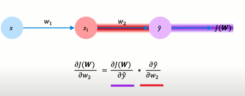
when computing the error for last layer we just compute the loss between the ground truth and the output of the models and then we need to evaluate the derivative of the loss over the weights, the derivative of the loss with respect to the weights of the last layer is simple:
$\frac{\partial L(x_{i})} {\partial w_{j}} = (\hat{y_{i}} - y_{i}) x_{ij}$
the problem is that i want to optimize the weights inside the neural network for which we do not have a $\hat{y_i}$ explicit. for do that i need to introduce an intermediate notation $a_{t} = \sum_{j} w_{jt}z_{j}$. We always some up the current input with the associated weights pass it to a non-linear function.
the loss $L$ depends on $w_{jt}$ only trough $a_{t}$:
$\frac{\partial L} {\partial w_{jt}} = \frac{\partial L} {\partial a_{t}} \frac {\partial a_{t}} {\partial w_{jt}}$
we can denote ${\partial a_{t}}$ with $\delta_{t}$, this can be computed with an iterative scheme, in the last layer $\delta_{t}$ is given by $(\hat{y_{i}} - y_{i})$ and in the hidden layers with a recursive formula to compute it (depends on the top layers). For any arbitrary units $z_{t}$ this unit send out to all the units $z_{s}$ (in the next layer) so for a generic units $a_{s}$ i can have that $a_{s}$ is connected to $a_{j}$ with the formula.
When i’m computing $\delta_{t}$ i’m summing up all the contributions of all the neurons in the next layer and i’m applying the chain rules. Once you have $\delta_{t}$ you start applying this rule and go back computing the propagation of all the layers.
$\delta_{t} = h^{‘}(a_{y}) \sum_{s \in S} w_{ts} \delta_{s}$
The derivative tells us the slope of the tangent line at any point along the curve; this slope of the tangent line tells us how quickly one variable is changing with resect to the other.
we want to find the weights and bias that minimize the cost functions; we are looking for the negative gradient of that function that tells how to change the w&b to best decrease the cost. Backpropagation is used to computed that gradient, the magnitude of each component into the gradient array tells how sensitive is the cost function is to each w&b. The cost of the function is more sensitive to more w&b rather than others.
looking at only one neuron, it is defined as $= \sigma (w_{0}a_{0} + w_{1}a_{1 + … + w_{n-1}a_{n-1}} + b)$; the activation of a single neuron is given by all the the neurons in the layer before (activations), the weights associated with each of these and a bias all passed trough a non-linear function.
We apply the chain rule backward from the loss to the input, we decompose the derivative into two terms; for the hidden layer have to apply the chain rule recursively.
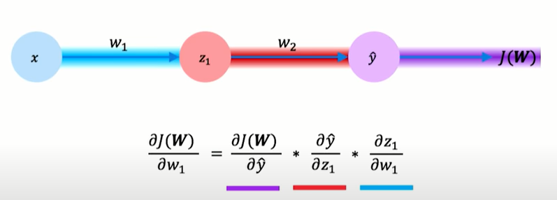
repeat this process for every weighting the network using gradients from later layers.
summary:
- For top layer i’m taking the local input and multiply by the local error that can be analytical computed
- For the previous layer and back i defined the $\delta_{j}$ and this delta is given by the local input and the local error
Using a general formulation we can define $w_{i \rightarrow j}$ (weights associated that goes from node i from node j), with $z_{i}$ is the local input and $\delta_{j}$:
$\frac{\partial L} {\partial w_{i \rightarrow j}} \delta_{j} z_{i}$
this operation is done in matrix form.
the backpropagation in the context of nn is all about assigning credit (or blame) for error incurred to te weights, there is an error that occurs at the last layer and this error depends on the input and on the current weights so we want to update the weights according to the influence that the weights have on the output. To perform this update we follow the path from the output to the input, se we find $\delta_{j}$ that correspond to the top of the network and we go back using the chain rules and once we get all the partial derivative corresponding to all weights we can apply gradient descent.
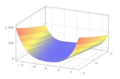
Minima
in In neural networks the optimization problem is non-convex, it probably has local minima. This prevent people to use neural network for long time, because they prefer methods that are guarantees to find the optimal solution.
Saddle points
Some directions curve upwards, and others curve downwards. At a saddle point, the gradient is 0 even if we are not at a minimum. If we are exactly on the saddle point, then we are stuck. If we are slightly to the side, then we can get unstuck.

Batch Gradient Descent vs Stochastic gradient descent vs Mini Batches
- In Batch Gradient descent we consider the entire dataset gradient at once. Basically i compute the summation of the gradient of the whole dataset, i apply some learning rate to it and i take the minus (since i want to go in the opposite site of the gradient). it is very stable butt need to compute gradients over the entire training set for one update (very computational expensive).
$\hat{g} \leftarrow + \frac{1}{N} \nabla_{\theta} \sum_{i} L ( f(x^{(i)}; \theta), y^{(i)})$
- in the Stochastic gradient descent (SGD) approach instead of using the entire dataset we sample each data point at the time an we update the weight for each sample (one data point per update). it is very noisy.
- SDG is suboptimal we want a trade off between SDG and BGD, this is the mini batches approach, using this approach the computation time per update does not depend on the number of training examples N, it allow computation on extremely large datasets (easy parallel implementation).
typically is hard to understand which Learning rate to use at the beginning, a common procedure is to start with a large lr and then decrease it trough the iteration using Learning rate schedule.
Optimizers
Momentum
Previously, the size of the step was simply the norm of the gradient multiplied by the learning rate. Now, the size of the step depends on how large and how aligned a sequence of gradients are. The step size is largest when many successive gradients point in exactly the same direction
What is the trajectory along which we converge towards the minimum with SGD? The momentum method is a method to accelerate learning using SGD; n the example SGD would move quickly down the walls but very slowly through the valley floor. Momentum simulates the inertia of an object when it is moving, that is, the direction of the previous update is retained to a certain extent during the update, while the current update gradient is used to fine-tune the final update direction. In this way, you can increase the stability to a certain extent, so that you can learn faster, and also have the ability to get rid of local optimization.
SGD suffers in the following scenarios:
- Error surface has high curvature
- We get small but consistent gradients
- The gradients are very noisy
for solving this problem we introduce a new variable $v$, the velocity. we think of $v$ as the direction and speed by which the parameters move as the learning dynamics progresses, it is an exponentially decaying moving average of the negative gradients.Doing this we take the history of the gradients so to have smooth way to update it.
- sample example from training set
- compute the gradients estimate $\hat{g} \leftarrow + \nabla_{\theta} L ( f(x^{(i)}; \theta), y^{(i)})$
- compute the velocity update $v \leftarrow \alpha v - \eta \hat{g}$
- apply update $\theta \leftarrow \theta + \alpha v$
The velocity accumulates the previous gradients and $\alpha$ is used to regulate the current current and the previous, if $\alpha$ is larger than the learning rate the current update is more affected by the previous gradients (usually is high around .8). Momentum is essentially a small change to the SGD parameter update so that movement through the parameter space is averaged over multiple time steps. Momentum speeds up movement along directions of strong improvement and helps the network avoid local minima.
Nesterov Momentum
Nestorov momentum is a simple change to normal momentum. The gradient term is not computed from the current position in parameter space but instead from an intermediate position. The idea is to first take a step in the direction of the accumulated gradient (lookahead step) and then calculate the gradient and make correction.
- sample example from training set
- update parameters $\tilde{\theta} \leftarrow \theta + \alpha v$
- compute the gradients estimate $\hat{g} \leftarrow + \nabla_{\tilde{\theta}} L ( f(x^{(i)}; \tilde{\theta}), y^{(i)})$
- compute the velocity update $v \leftarrow \alpha v - \eta \hat{g}$
- apply update $\theta \leftarrow \theta + \alpha v$
- This helps because while the gradient term always points in the right direction, the momentum term may not.
- If the momentum term points in the wrong direction or overshoots, the gradient can still “go back” and correct it in the same update step.
The difference between Nesterov momentum and standard momentum is where the gradient is evaluated. With Nesterov momentum, the gradient is evaluated after the current velocity is applied. Thus one can interpret Nesterov momentum as attempting to add a correction factor to the standard method of momentum.
we end up trusting more the gradient and less the momentum.
Adaptive Learning Rate Methods
the core idea is that there are some features (w&b) that are more important than others, so we should treat them differently. The intuition behind AdaGrad is can we use different Learning Rates for each and every neuron for each and every hidden layer based on different iterations.
Another problem is that the same learning rate is applied to all parameter updates. If we have sparse data, we may want to update the parameters in different extent instead.
Adaptive gradient descent algorithms such as Adagrad, Adadelta, RMSprop, Adam, provide an alternative to classical SGD. These per-parameter learning rate methods provide heuristic approach without requiring expensive work in tuning hyperparameters for the learning rate schedule manually.
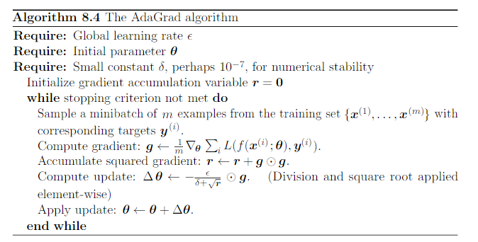
Adagrad
The AdaGrad algorithm individually adapts the learning rates of all model parameters by scaling them inversely proportional to the square root of the sum of all the historical squared values of the gradient.
The parameters with the largest partial derivative of the loss have a correspondingly rapid decrease in their learning rate, while parameters with small partial derivatives have a relatively small decrease in their learning rate. The net effect is greater progress in the more gently sloped directions of parameter space
Empirically, however, for training deep neural network models, the accumulation of squared gradients from the beginning of training can result in a premature and excessive decrease in the effective learning rate.
it downscale a model parameter by square-root of sum of squares of all its historical values. Adagrad performs larger updates for more sparse parameters and smaller updates for less sparse parameter. It has good performance with sparse data and training large-scale neural network. However, its monotonic learning rate usually proves too aggressive and stops learning too early when training deep neural networks.
the main problem with adagrad is that the operation can be too aggressive. AdaGrad perform a premature and excessive decrease in the effective learning rate; AdaGrad might shrink the learning rate too aggressively, we want to keep the history in mind. (no need to manually tune the LR).
RMSProp
To solve the problem of the aggressivity of Adagrad with RMSProp by changing the gradient accumulation into an exponentially weighted moving average.
AdaGrad shrinks the learning rate according to the entire history of the squared gradient and may have made the learning rate too small before arriving at such a convex structure. RMSProp uses an exponentially decaying average to discard history from the extreme past so that it can converge rapidly after finding a convex bowl.
- sample example from training set
- compute the gradients estimate $\hat{g} \leftarrow + \nabla_{\tilde{\theta}} L ( f(x^{(i)}; \tilde{\theta}), y^{(i)})$
- Accumulate: $r \leftarrow \rho r + (1 - \rho) \hat{g} \odot \hat{g}$
- apply update $\theta \leftarrow \theta + \alpha v$
the decay parameter $\rho$ tells if we have to count more on the history or to the current value. RMSprop adjusts the Adagrad method in a very simple way in an attempt to reduce its aggressive, monotonically decreasing learning rate.
We can also use RMSProp with Nestorov momentum, just using that procedure.

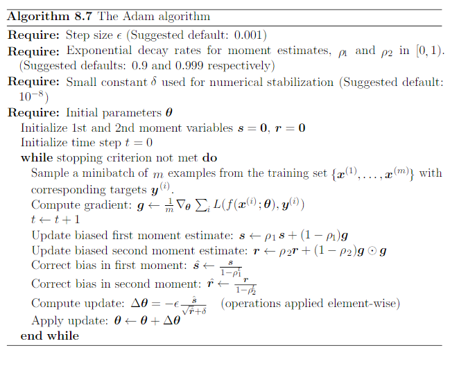
ADAM Adaptive Moments
Adam is like RMSProp with Momentum but with bias correction terms for the first and second moments, The bias correction compensates for the fact that the first and second moments are initialized at zero and need some time to ‘warm up’.
First, in Adam, momentum is incorporated directly as an estimate of the first-order moment (with exponential weighting) of the gradient. Second, Adam includes bias corrections to the estimates of both the first-order moments (the momentum term) and the (un-centered) second-order moments to account for their initialization at the origin
Batch Normalization
Normalization mean collapse inputs between 0 and 1 while standardization means make the data with mean equal to 0 and variance equal to 1.
Batch normalization provides an elegant way of reparametrizing almost any deep network. The reparametrization significantly reduces the problem of coordinating updates across many layers.
As learning progresses the distribution of internal layer inputs changes due to parameter updates, this can result in most inputs being in a nonlinear regime and slow down learning. This phenomenon is know as internal covariate shift (change in the distribution of inputs during training).
To solve this problem we can use Batch normalization which is a method to parametrize a deep network, it can be applied to the input layer or any hidden layer.
We can understand this process considering the following example:
$H =
\begin{matrix}
h_{11} & h_{12} & … & h_{1N}
h_{21} & h_{22} & … & h_{2N}
h_{M1} & h_{M2} & … & h_{MN}
\end{matrix}$
where each row represents all the activations in a layer, the main idea is to replace $H$ with:
$H^{‘} = \frac {H - \mu} {\sigma}$
where $\mu$ is mean of each unit and the $\sigma$ standard deviation (they are vector computed over columns of $H$).
using batch norm we improve gradient flow trough the network, allowing higher learning rates and reducing the strong dependencies on the initialization of w&b.
batch norm allow faster training since it avoid that some change in the features can cause a very high loss increase. Decrease the importance of the initial weights and lastly regularizes the model.
Anyway standardizing the output of a unit can limit the expressive power of the neural network, the idea to solve this problem is to introduce scale and bias that are also learned with backpropagation ending up with:
$\gamma H^{‘} + \beta$
We have to value that have been standardize and we multiply it by the scale and the offsets that are two trainable parameters.
normally batch normalization layers are inserted after convolutional or fully connected layers and before the non-linearity.
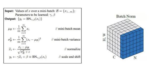
assume the batch size is 3, we pass the sample and we know the activation of a neuron for the 3 images; we can calculate easily the mean of the standard deviation. We standardize the data subtracting the mean and dividing by the sd. But the mean and the sd computed are too much dependent on the batch so we introduce the scale and bias that are two learnable parameters that should approximate the real mean and sd of the data.
we also have different wat of normalization for instance the layer normalization which is widely used in transformers in which we directly estimates the normalization statistics from the summed inputs to the neurons within a hidden layer
Regularization
The central challenge in machine learning is that our algorithm must perform well on new, previously unseen inputs. The ability to perform well on previously unobserved inputs is called generalization. We generally assume that the training and test examples are independently drawn from the same data distribution, this property is called i.i.d. independent and identically distributed.
The factors determining how well a machine learning algorithm will perform are its ability to: Make the training error small and Make the gap between training and test error small.These two factors correspond to the cases of underfitting and overfitting. We can control overfitting/underfitting by altering the model capacity (which is the ability to fit a wide variety of functions).
in order to avoid overfitting, if there is the possibility, we can use more data to train the model, use models with right capacity and ensembles different models (using bagging) but if there is no room for this approaches we can use different and more advance techniques such as regularization.
We are interested into regularization methods for deep architectures. Deep learning algorithms are typically applied to complicated domains (e.g. images, sequences). Thus, controlling the complexity of the model is not a simple matter of finding the model of the right size. Instead, in practical applications we almost always find that the best model (the one that minimize the generalization error) is a large model that has been regularized appropriately.
Using NN the overfitting problem is serious, we have NN that have millions of parameters and situations in which the dataset is smaller than the number of parameters. Overfitting in neural networks can be controlled in many ways:
- Architecture: Limit the number of hidden layers and the number of units per layer.
- Early stopping: Start with small weights and stop the learning before it overfit.
- Weight-decay: Penalize large weights using penalties or constraints on their squared values (L2 penalty) or absolute values (L1 penalty).
- Noise: Add noise to the weights or the activations.
Simple speaking: Regularization refers to a set of different techniques that lower the complexity of a neural network model during training, and thus prevent the overfitting
Parameter Norm Penalties
We can limit the model capacity by adding a parameter norm penalty to the objective function:
$\tilde{L} ( \theta) = L(\theta) + \lambda \Omega(\theta)$
where the norm penalty $\Omega$ that penalizes only the weights of the affine transformation at each layer and leaves the biases un-regularized (It would be desirable to use a separate penalty with a different $\lambda$ coefficient for each layer of the network. But search for the correct value of multiple hyperparameters can be expensive. In practice, the same value is used).
L2 Norm (Ridge)
Most important (or most popular) regularization is the L2 norm were we penalized on the square of the weights such as:
$\tilde{L} = \sum_{i=1}^{N} L(f(x_{i}, \theta), y_{i}) + \frac{\lambda}{2} \sum_{l} \left \Vert w_{l} \right \Vert ^{2}$
The L2-regularization can pass inside the gradient descent update rule and it is also called weight decay since it force the weights to be small. The only difference is that by adding the regularization term we introduce an additional subtraction from the current weights (first term in the equation). In other words independent of the gradient of the loss function we are making our weights a little bit smaller each time an update is performed.
L1 Norm (Lasso)
In the case of L1 regularization (also knows as Lasso regression), we simply use another regularization term $\Omega$. This term is the sum of the absolute values of the weight parameters in a weight matrix:
$\tilde{L} = \sum_{i=1}^{N} L(f(x_{i}, \theta), y_{i}) + \frac{\lambda}{2} \sum_{l} \left \Vert w_{l} \right \Vert$
The derivative of the new loss function leads to the following expression, which the sum of the gradient of the old loss function and sign of a weight value times alpha.
In the case of L2 regularization, our weight parameters decrease, but not necessarily become zero, since the curve becomes flat near zero. On the other hand during the L1 regularization, the weight are always forced all the way towards zero.
Data Augmentation
Best way to make a ML model to generalize better is to train it on more data, in practice amount of data is limited but we get around the problem by creating synthesized data.
Data set augmentation very effective for the classification problem of object recognition, images are high-dimensional and include a variety of variations, may easily simulated. Translating the images a few pixels can greatly improve performance. (Not apply transformation that would change the class: OCR example: ‘b’ vs ‘d’; some transformations are not easy to perform).
Noise as Regularizer
For some models, the addition of noise with infinitesimal variance at the input of the model is equivalent to imposing a penalty on the norm of the weights. In the general case, it is important to remember that noise injection can be much more powerful than simply shrinking he parameters, especially when the noise is added to the hidden units.
Injecting noise at the output targets
Most datasets have some number of mistakes in they labels. It can be harmful to maximize $log p(y | x)$ when $y$ is a mistake. One way to prevent this is to explicitly model the noise on the labels. For example, we can assume that for some small constant $\eta$, the training set label $y$ is correct with probability $1 - \eta$ , and otherwise any of the other possible labels might be correct.
This assumption is easy to incorporate into the cost function analytically, rather than by explicitly drawing noise samples. For example, label smoothing regularizes a model based on a soft-max with $k$ output values by replacing the hard 0 and 1 classification targets with targets of $\frac{\eta}{k-1}$ and $1 - \eta$ , respectively.
Early Stopping
Procedure: Start with small weights and stop the learning before it overfit. Every time the error on the validation set improves, we store a copy of the model parameters. When the training terminates, we return these parameters, rather than the latest parameters.
Multi-Task Learning
Multi-task learning is a way to improve generalization by pooling the examples out of several tasks. Different supervised tasks share the same input $x$, as well as some intermediate-level representation $h^{(shared)}$
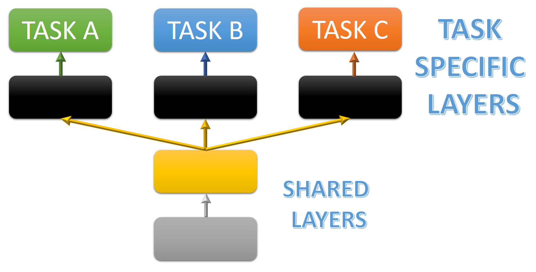
While performing multi-tasking learning we will have two different family of parameters:
- Task specific parameters: Which only benefit from the examples of their task to achieve good generalization, These are typically the upper layers of the neural network.
- Generic parameters: Shared across all tasks, which benefit from the pooled data of all tasks (typically first layers).
We can enforce some parameters inside the network to be exactly the same: parameter sharing. A significant advantage of parameter sharing over regularizing the parameters to be close is that only a subset of the parameters (the unique set) needs to be stored in memory.
Soft constraints: Parameter Tying
Instead of enforcing same parameters we can enforce soft constraints, in the sense that certain parameters should be close to one another (MMD in deep domain adaptation).
Extensive use of parameter sharing occurs in convolutional neural networks (CNNs) applied to computer vision. Convolutional neural networks are multi-layer networks with local connectivity: neuron in a layer are only connected to a small region of the layer before it, there is this sharing of weight of parameters across spatial positions this allow to learning shift-invariant filter kernels and to reduce the number of parameters.
Model Ensembles and Dropout
the ensembles of models implies train several different models separately, then have all of the models vote on the output for test examples so to average it (typically not done with neural nets).
the Dropout is a more efficient way to regularize the models, when apply dropout we randomly set some neurons to zero in the forward pass. The choice of units to drop is random, determined by a probability p, chosen by a validation set or set a priori. Dropout is very useful since it forces the network to have redundant representation of the most important features.
Dropout provides an inexpensive approximation to training and evaluating a bagged ensemble of exponentially many neural networks, Dropout training is not quite the same as bagging training. In the case of bagging, the models are all independent. In the case of dropout, the models share parameters, with each model inheriting a different subset of parameters from the parent neural network. This parameter sharing makes it possible to represent an exponential number of models with a tractable amount of memory.